Accuracy and Checking in FEA Part 2
Let's take a closer look at finite element analysis model checking aspects, including supplementary or auxiliary analyses set up to confirm correct model behavior.


Latest News
February 1, 2014
By Tony Abbey
| Read Part 1 ofAccuracy and Checking in FEA here. |
Editor’s Note: Tony Abbey teaches live NAFEMS FEA classes in the US, Europe and Asia. He also teaches NAFEMS e-learning classes globally. Contact [email protected] for details.
Before a production run, we do special auxiliary finite element analysis (FEA), including analyses for normal modes and thermal soak. These processes are not designed to give us final answers, but to give us confidence in the analysis model. They are straightforward to set up, and only require a few extra physical properties to be defined.
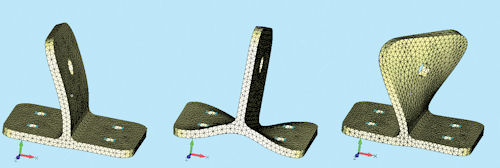 Fig 1: Three modes of a correct model. |
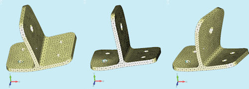 Fig 2: Three modes of an incorrect model. |
There are two ways we can carry out a normal modes check analysis. The first is intuitive, and looks at the frequencies and mode shapes of the grounded structure. We can ignore any loading applied to the model, as the normal modes analysis is exploring the load-independent resonant frequencies of the model. That is useful to us because the mode’s shapes and frequencies can uncover a variety of modeling errors. The only data change is to define material density, to allow calculation of mass.
Fig. 1 shows a typical result, with each mode animated in turn. Mode shapes highlight any unusual response in the structure, such as parts that seem to flap in the breeze, show apparent cracks opening and closing, or that seem strangely stiff. Fig. 2 shows an example highlighting a badly connected component caused by a modeling error.
The frequency of each mode is expressed in cycles per second or Hz. It is proportional to the square root of the stiffness contribution divided by mass contribution of that mode. Simple hand calculations, or FEA unit load cases can calculate the stiffness contribution of each mode. The modal effective mass table will give us the appropriate mass contribution.
Alternatively, we can compare against test results. However, we should have a general feel for what the natural frequencies of the structure will be, so all we are doing a ballpark check. A structure with a first natural frequency of 1,000 Hz, for example, is very stiff. If occurring in a bridge, ship or aircraft model, then we have made a mistake, probably associated with units. This type of structure should have primary frequencies of the order 2 to 10 Hz. So if your gearbox housing, conrod or mobile phone case model is this low, there is a problem.
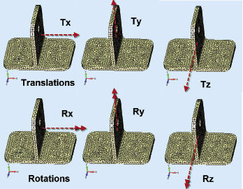 Fig 3: Rigid body modes of a structure. |
I recommend this form of checking to everyone, but there is a more rigorous extension of this. In this case, the model is disconnected from ground and allowed to float free. Again, this seems a little bizarre, but what we are after are the rigid body modes of the structure.
Fig. 3 shows the six rigid body modes of a typical structure if modeled correctly. Less than six indicates some form of cross coupling error; each count above six indicates a spurious mechanism. My personal record is around 800!
Each rigid body mode will have a frequency close to zero, typically below 1.0E-4 Hz. We use a strain energy contour plot on each mode to ensure the strain energy is zero in each case. Any non-zero strain energy indicates some part of the structure is badly connected or numerically unstable. Mode 7 should be the first elastic mode with significant strain energy present.
Normal modes analysis is able to solve for actual rigid body modes or spurious mechanisms. This means it is a powerful technique to search for this type of error, which will usually cause a linear analysis to fail.
Auxiliary Thermal and Gravity Analyses
With these processes, the constraints to ground are again removed and a set of minimum constraints is provided. The minimum number of degrees of freedom (DOF) required to constrain out rigid body motion is 6. In other words, three nodes have 3, 2 and 1 DOF constraints applied to each respectively. I will describe this in detail in a future article, but for the moment, follow the scheme shown in Fig. 4.
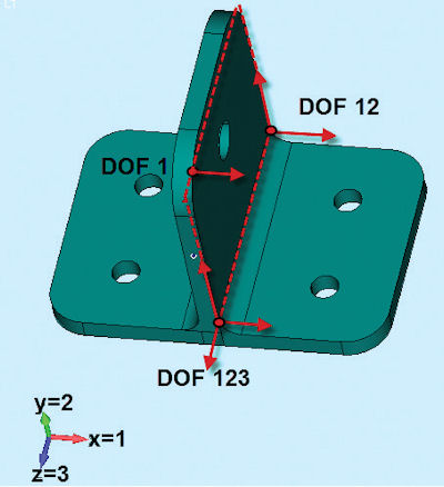 Fig 4: Minimum constraint set with 6 DOF defined. |
The coefficient of thermal expansion (CTE) is applied to every part of the structure. For this check, it is important to apply just a single CTE and ignore any variation in material. A thermal analysis is carried out on the structure, with an arbitrary temperature change defined. This simulates a structure hung in space by fine wires and heated up from room temperature uniformly. A real test should give a free thermal expansion of the structure. This is also the analysis objective. Any localized stress indicates modeling errors—as seen in the top image of Fig. 5, where a rigid element is defined incorrectly. Stresses are close to zero as the structure is free to expand, as shown in the lower image in Fig. 5.
The gravity checks use three load cases, with a unit of gravity applied in each of the directions X, Y and Z. A gravity load in FEA is a form of “body” load, requiring the definition of gravity direction and magnitude. Every element has a volume and corresponding density, and hence a mass. Element nodal forces balance the applied acceleration. The model gets a good workout, as no element escapes the attentions of the gravity loading.
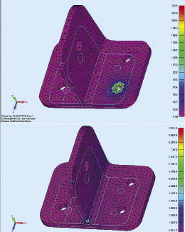 Fig 5: Free thermal expansion check: Incorrect upper and correct lower, with negligible stress. |
The first check makes sure that the total applied force created in each case balances total reaction force. The next check is on the rounding error reported by the solver for each of the three load cases. The format of the rounding error varies among solvers, but reports the accuracy of the stiffness matrix inversion.
Finally, we can animate the deformed shape plot to check for any unusual behavior, in a similar way to the modal check. I strongly recommend animating mode shapes, as the eye catches unusual motion much more easily than a static plot.
Solver Checks
We have looked at auxiliary analysis running solver checks for numerical stability and numerical accuracy using the load balance and load residual. The production analysis is also checked.
Part one of this article (see the January issue of Desktop Engineering) discussed preprocessor element geometry checks. A preprocessor may have a different geometry definition from a solver, so we look for any inconsistencies in error checking.
Before opening the full postprocessor—and spending time and resources in loading large models—it is worth doing sanity checks on maximum stresses and displacements. In most cases, it is possible to set up a small text output stream or request an output window that just contains this data.
It is better to spot now that part of the structure has moved 27.8 km or has a peak stress of 4,000 MPa rather than after all of the result data has been read into the postprocessor.
Postprocessing Checks
Finally, we can do postprocessing checks on element results. That’s often when the real detective work begins. (Remember that every analysis is guilty until proved innocent.)
In previous articles I have discussed how the traditional FEA method solves for displacements rather than stresses. This has a significant effect on the way that we should be considering stresses in the postprocessor. The displacement field throughout the structure should be continuous—and with a fine enough mesh, it should be a good representation of the actual structural deflections. However, the stress throughout the FEA model is probably not continuous. Each element back-calculates its own stress distribution independently from the common displacement field.
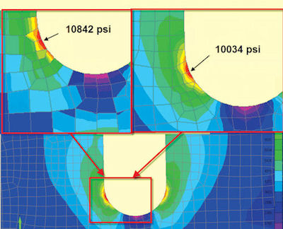 Fig 6: The effect of stress averaging. |
This means that Element A, which is a neighbor to Element B, calculates its internal element stresses and extrapolates to its nodes—with no reference to Element B. The shared nodes between A and B may well have different contributions coming from each element, as Fig. 6 shows.
If we allow the postprocessor to use nodal stress averaging on the raw data coming from the FEA solver—the data from A and B nodes independently—we will have an inaccurate and possibly non-conservative result for stresses. Nodal stress averaging should always be switched off when checking for peak stress values.
If accurate peak stress values are critical, it is always a good idea to do a convergence study. This means running the model with increased mesh density in the area of interest. We don’t have to globally refine the mesh throughout the structure; that is usually prohibitive.
Instead, focus on the key areas for speed and efficiency. Fig. 7 shows a finer mesh run to confirm whether the initial results are conservative. The initial mesh had, in fact, reached a converged value. A subsequent nonlinear analysis was needed to show that the stresses were within limits.
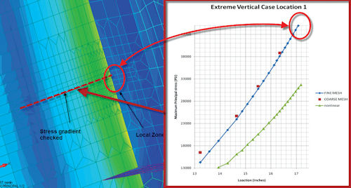 Fig 7: Mesh convergence check at a stress concentration. |
We should always review the regions of peak stress to make sure that there is a physical reason for their presence, rather than modeling errors. A real structure has no peak stress unless there is a local load, constraint or change in material or section. A spurious peak stress could mean modeling errors—including reversed pressure loading, spurious constraints, poor local meshing, etc.
Understand the Stresses
Understanding why and how the structure is responding to the loading and constraint environment is important. This is a complicated task requiring some experience. I’ll be providing some hints and tips in a future article, but for now, consider the type of stress to check. Von Mises stress indicates whether the structure is operating above the yield limit. This is useful to see where the structural “hotspots” are.
On the other hand, the Von Mises stress masks the nature of the stress that we are seeing. Is it a tensile or compressive stress state, with implications for fatigue loading and buckling? Is the stress state dominated by direct or shear stresses? Shear stresses are always a major concern, as they are the most damaging form of stresses in general.
Plotting component stresses and principal stresses around the hotspot regions reveals the stress state and allows a more pragmatic redesign if required.
The key to a good structural analysis is in gaining an understanding of the structural load paths and stresses that are being developed. This will show through in any report presentation and will give everyone a sense of confidence in your analysis work.
Tony Abbey is a consultant analyst with his own company, FETraining. He also works as training manager for NAFEMS, responsible for developing and implementing training classes, including a wide range of e-learning classes. Send e-mail about this article to [email protected].
Subscribe to our FREE magazine, FREE email newsletters or both!
Latest News
About the Author
Tony Abbey is a consultant analyst with his own company, FETraining. He also works as training manager for NAFEMS, responsible for developing and implementing training classes, including e-learning classes. Send e-mail about this article to [email protected].
Follow DE

