Fig. 1: Typical geometry of a shoulder fillet.


May 1, 2017
Editor’s Note: Tony Abbey teaches live NAFEMS FEA classes in the U.S., Europe and Asia. He also teaches NAFEMS e-learning classes globally. Contact [email protected] for details.Are the Stresses Real or Imagined?
Local design features, under applied loading, often result in an increase in local stress. Often the stress levels will dominate any strength analysis we carry out using finite element analysis (FEA). A theme occurring throughout my DE articles has been the requirement for these stresses to be as accurate as possible. In this article, I take a closer look and review the background to the accuracy objective. Do the local stresses really matter from a physical and compliance point of view?
 Fig. 1: Typical geometry of a shoulder fillet.
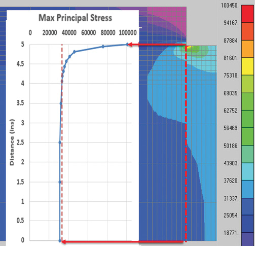 Fig. 2: Stress variation across shoulder with eight elements on edge.
In some circumstances, the stress levels that we predict from FEA are not physically meaningful. The stress distribution and high levels of stress locally can be described as an FEA “artifact.” The most common examples of where this can happen are the following:
- applying a point load;
- creating abrupt local transitions in local loading;
- constraining a model at a point;
- creating abrupt transitions in local constraints;
- abrupt transition between materials; and
- sharp re-entrant corners.
Fig. 2 shows the stress variation for a model with eight elements along each local edge adjacent to the right angle. A peak stress of 100,450 psi occurs. Notice how localized this stress peak stress region is. The average stress across the bulk of the section is around 31,000 psi. The peak stress can be quoted as a stress concentration factor, Kt. Kt is defined as the ratio of peak stress to nominal stress. The nominal stress is defined as the applied load divided by the narrow cross-sectional area. It is important to realize that the nominal stress is not a “real” stress. It is an effective baseline stress, which ignores the influence of any local stress-raising feature. In this case the nominal stress is calculated as 33,335 psi, giving a Kt of 3.01.
Fig. 3 shows the peak stresses in the corner for a range of mesh sizes, from one element on edge to 60 elements on edge. The element edge axis is plotted on a log scale. The value of peak stress is totally dependent on the level of mesh density around this region. At 60 elements on edge, the peak stress is 220,213 psi and the Kt value is 6.61. The average stress distribution in the bulk of the cross-section remains the same. It is only the very local peak stress (and hence stress gradient) that is increasing. There is no sign of any convergence, as shown in the log-linear scales of the plot. Essentially, we will get an infinite stress as the number of elements increases to infinity.
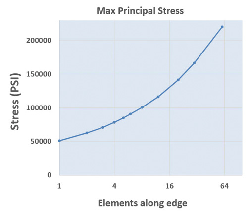 Fig. 3: Convergence study for the right angle model.
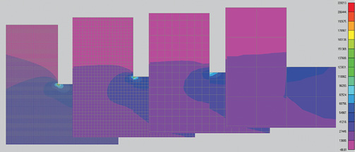 Fig. 4: Stress distributions for the right angle model.
This is a warning sign that our FEA model is not physically meaningful. An FEA model should always converge to a stress level. We have stumbled into a stress singularity. Classical elasticity theory can also be used to solve simple geometric problems like this. In fact, the handbooks of Kt values for standard geometries are based on this type of calculation. It turns out that these solutions also result in conflicting assumptions at the corner of the feature, where theoretically the stresses go off to infinity. In the limit, at very small load levels, stresses will exceed yield. This is obviously completely fictitious. By de-featuring the fillet radius, we have removed any possibility of getting an accurate prediction for what the peak stress would be in this region.
Fig. 4 shows that this is very much a localized problem. The stress contours have been fixed at the maximum stress 220,213 psi, across all of the results for mesh size of 2, 8, 20 and 60 elements on edge.
Stress Concentration: Modeling the Fillet
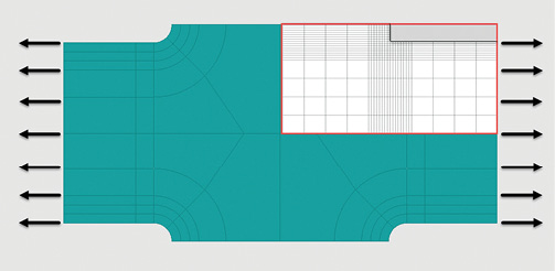
The filet region with 1.0-in. radius is now modeled. The quarter symmetry mesh is shown in Fig. 5.
A series of analyses are carried out with increasing mesh density. The geometry is divided up into sectors so that careful control of the mesh and element shape is possible. One challenge of a good mesh convergence study is to keep the element shapes consistent. An arbitrary mesh will give changing aspect ratios, internal angles, etc. in the local elements and distort convergence trends.
Fig. 6 shows the results of the study. The curve labeled “1.0 Fillet” shows that the stress peak converges to a value of 65,600 psi at around 10 elements per edge, where the edge is defined as a 45° arc of the fillet. This allows broadly the same x-axis to be used for both the filleted and right angle model. A line is drawn on the graph to indicate the converged stress result. The converged Kt value is 1.97. The right angle model results are overlaid and labeled as such. As before, there is no convergence for this model.
The stress patterns for increasing mesh density are shown in Fig. 7, with a common contour range, set to the peak value of 65,600 psi. The convergence to the peak value can be seen across the plots. The location of the peak value also migrates around the fillet arc slightly. The coarser meshes are unable to give sufficient fidelity to locate its position accurately. Again, the area is extremely localized.
Reconciling Right Angle and Filleted Models
It is sometimes held to be true that a de-featured model such as the right angle model can give reasonable stress results if the element size can be tuned to a characteristic length. In Fig. 6, the right angle study intersects the converged solution at two elements per edge. We could argue that around two elements per edge on the right angle model would give the “correct” stress to match the filleted model converged results. I really don’t buy into this approach as it takes a lot of data fitting to get a similitude between the actual mesh and defeatured mesh results. The only merit would be where a particular range of components is regularly analyzed and careful correlation can be made. The de-featured tuned mesh can then be used as a surrogate. A 2D study could save a lot of expensive fine mesh 3D modeling.
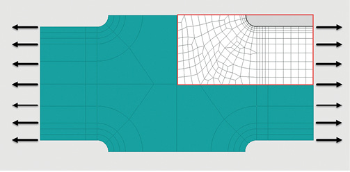 Fig. 5: Geometry and mesh of filleted model.
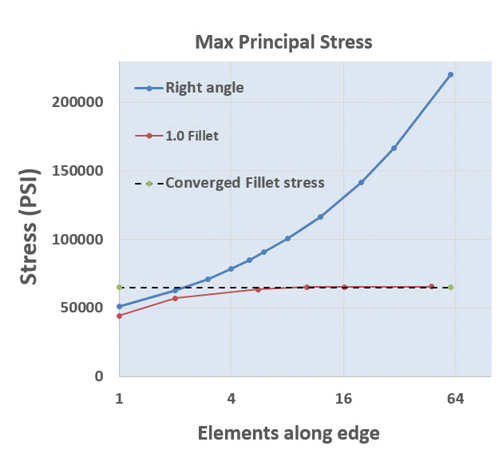 Fig. 6: Convergence study for the filleted model.
 Fig. 7: Stress distributions for the filleted model.
However, in a general case, the actual stress concentration peak is unknown, and there is not much alternative to doing a convergence study. One of the trends in commercial FEA meshers has been for default mesh density to increase. This means that a typical edge count of two is now perhaps eight. In turn, this means that a sharp corner like ours will see 100,000 psi rather than a “comfortable” 65,600 psi. Neither value has any merit, but these types of stress predictions are often used. Over the course of 10 years, a typical mesh may be at a 32 count and give 175,000 psi. This will perhaps serve to make the need for accurate modeling more obvious as the spurious high stresses are increasingly unacceptable in design.
To some extent we have had a “serendipity” effect for many years. A poorly detailed feature with an inadequate mesh has given stress levels that seem, by intuition, to be of the right order.
Does Stress Concentration Accuracy Matter That Much?
If we assume that including the geometric feature is important, so that at least we can get some order of accuracy, then the next question is how accurate do we have to be? The answer depends on the type of failure we are trying to predict and the behavior of the material.
For a strength analysis on a ductile material, traditionally only nominal stresses were calculated and reserve factors or margins of safety on limit load were based on this. The justification was always that very localized peak stress regions would yield and self-relieve. The conclusion for an FEA result, following on from the hand calculation approach, should perhaps be similar; we can ignore the localized stress and deal with nominal stresses. In the case of the fillet feature discussed here that would mean using 33,335 psi as found in the main body of the shoulder. However, with FEA, we can raise our game, and with a little extra effort get a converged stress concentration result. Now we can see a stress representation that was impossible in hand calculations. We should get reasonable accuracy via a stress convergence study and then we can decide what engineering assessment to make of that stress level. If we subsequently choose to ignore local stress concentrations, we do so on the basis of knowing their value and distribution.
If we are concerned about ultimate loading, then we can take a different approach. Hand calculations use form factors and other methods to correlate test results with simple elastic calculations. In FEA we can use nonlinear analysis to investigate further what a nonlinear relationship is. It is very difficult to model failure, but we can move toward ultimate loads. In this case, we need a very fine mesh model to track the growth of plasticity and the development of geometrically nonlinear internal forces. Good mesh convergence on a linear analysis would be a first stage in this type of analysis.
For a strength analysis on a brittle material, we need to have very accurate mesh convergence proven. There is no demonstrable margin between yield and ultimate failure. Therefore, the peak stress at the stress concentration will dictate the final failure margin. We also should not be de-featuring in this case.
For a fatigue analysis, we also need to have very accurate stresses. The stresses will be directly used in a high cycle fatigue calculation and converted to equivalent strains in a low cycle fatigue calculation. As an example, assume that the shoulder is loaded with a fully reversed cyclic loading with a stress amplitude of 65,600 psi (converged mesh value) at the stress concentration region. Assuming a medium strength steel and no environmental corrections, the life would be 221,000 cycles. If the very coarse mesh of two elements per arc is used, then the peak stress is 57,800 psi and the life would be over 1 million cycles. A medium accuracy mesh of six elements per arc gives a peak stress of 63,700 psi, resulting in a life of 315,000 cycles. It is clear that the fatigue life is very sensitive to the accuracy of the stress calculation.
The effect of a stress concentration on fatigue life is actually subtler than this. Low strength steels are not as fatigue sensitive as the stress concentration factor, Kt, would suggest. From experimental evidence a reduced factor Kf (fatigue notch factor) is used to better correlate with test. However, we have to start with an accurate estimate of Kt (or the stress gradient at the peak). The reduction in effectiveness follows as part of the fatigue life calculation.
There is a strong temptation to either de-feature or mesh poorly at geometric stress raisers. Many failure predictions do require accurate stresses with evidence of a good convergence study. Even in the case of ductile materials being assessed against limit loading, it is useful to know the stress peaks and distribution of high stresses—even if subsequent engineering judgment can discount them.
Subscribe to our FREE magazine, FREE email newsletters or both!
About the Author
Tony Abbey is a consultant analyst with his own company, FETraining. He also works as training manager for NAFEMS, responsible for developing and implementing training classes, including e-learning classes. Send e-mail about this article to [email protected].
Follow DE

