Fig. 6: A global/local analysis of a ship.


Latest News
September 1, 2014
Editor’s Note: Tony Abbey teaches live NAFEMS FEA classes in the US, Europe and Asia. He also teaches NAFEMS e-learning classes globally. Contact [email protected] for details.
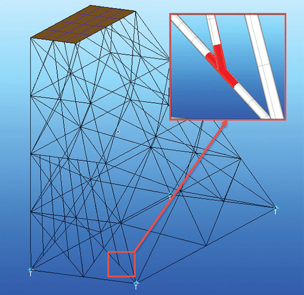 Fig. 1: Global model of an oil rig, showing joint of interest.
One of our major concerns in finite element analysis (FEA) is the required computing resource, including the time taken to run the analysis and the amount of memory it will use. We want answers in hours, not days and we want to solve within core RAM and not spill to virtual memory or physical disk, either of which will slow down the solution.
Techniques have evolved within FEA to reduce computing resources. These techniques still remain valid in modern analyses, as there is a natural tendency to use larger and more complex FEA simulations, as more resource becomes available.
In Situ Local Modeling
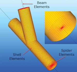 Fig. 2: Detail of local shell model connection into global beam model.
This approach positions the high-fidelity local model directly within the overall global model—that is, in situ. The analysis uses a single run with full connectivity between the model zones. The advantage lies in avoiding user interpolation of boundary displacements or forces from the global to local models. The disadvantage is that we introduce connection elements between the two models.
Fig. 1 shows an oil rig jacket modeled globally using beam elements. The joint is investigated for local stress concentrations. Beam elements cannot simulate the load path, and thus there are stresses locally across the joint between two members. All the load transfer in the beam element model takes place at the single nodal connection. The real load transfer is via the welded intersections of the cylinders, with resulting local stress concentrations.
To model the joint in detail, improved representation is made with a local shell model, shown in Fig. 2. This could be a local solid model if required. The shell or solids develop the correct load transfer path in the walls between the intersecting cylinders and stress concentrations at the intersections. The computing resource for a local/global model is much less than a full high-fidelity model.
Here, “spider” elements are used to connect the shell mesh and the beam mesh. This is a term used for this type of connectivity element. There are two variations of the spider:
- An infinitely stiff spider will make the connection between the beam end and shell cylinder free end fully rigid, so the cross-section cannot ovalize or move out of its original plane.
- A perfectly flexible spider will allow the shell cylinder to ovalize and distort out of plane.
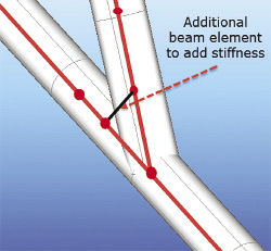 Fig. 3: Compensating for beam joint stiffness by adding a linking beam.
As an aside, it is interesting to compare the stiffness of the beam model and the shell model. The beam model is not stiffened by the presence of the intersecting beam walls, as would happen in reality. All stiffness is developed at the common single node “joint.” Many analysts introduce a short connecting beam across the two main beams, as shown in Fig. 3. There is no exact way to define the properties and location of this adjusting element, but a rule of thumb would be to use the smallest pipe section and run the element through the intersection location.
An alternative for joining dissimilar element types or mesh sizes is to use a linear, or “glued” contact method. Contact methods have been developed over many years in nonlinear analysis to simulate components striking one another, bearing surfaces in lugs and pins and many other applications. The contact stiffness that is developed when surfaces mate can be used in a linear analysis—if it is assumed the contact is always present and forms a constant load path. The advantage is that we can connect dissimilar meshes together with a reasonably compliant contact stiffness.
Fig. 4 shows a dissimilar mesh used to put a high-fidelity local model into the region around a hole in a plate. This is an alternative to the usual approach of refining the mesh continuously from the coarse mesh region. The arbitrary zone we are considering as the local model is shown within the square. The stress contour pattern results in a comparative coarse continuous mesh.
To set up the global/local model, the inset square around the whole is cut out and meshed with much higher fidelity. This is the local model. It is placed within the remaining global model, and the two are connected together using linear contact. The resulting stress distribution in the fine mesh is shown in Fig. 5(b), and can be compared to the stress distribution of the original mesh shown in Fig. 5(a).
The glued contact method is extremely effective in enabling an in situ global/local modeling technique. There are many other applications. Fig. 5(c) shows an alternative hole configuration—in this case an ellipse, substituted via a new local model into the original global model.
The accuracy of the in situ global/local model using either of these techniques depends on how well the transition region (either connector elements or linear contacts) represents stiffness and load transfer path. The stresses in the transition zone are always suspect, so we ensure that this region is away from the stress concentration region of interest.
One rule of thumb is to consider a critical dimension, such as the hole radius or the pipe diameter, and set the transition region at least twice this distance. I have about three diameters on the pipe model, but only half the diameter in the hole model, for example. The justification is that stress concentrations in this configuration are known to be very local.
Independent Local Modeling
An alternative to in situ local modeling is to run the analysis in two stages. The local zone to be investigated is identified within a global model. This is important, as it allows nodes and elements to be aligned on the subsequent boundary between the global and local models. The global model is run, and either the nodal forces or nodal displacements are extracted from the boundary. The local model is then run, using the boundary conditions extracted from the global model. The objectives are typically as before—a high-fidelity mesh in a local region or a change in structural configuration in a local region.
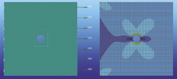 Fig. 4: Comparative model with a coarse mesh and no local model.
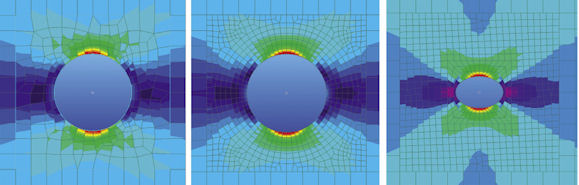 Fig. 5: From left: (a) peak stresses in the coarse mesh, (b) peak stresses in the fine mesh local model, (c) an ellipse replacing the circle.
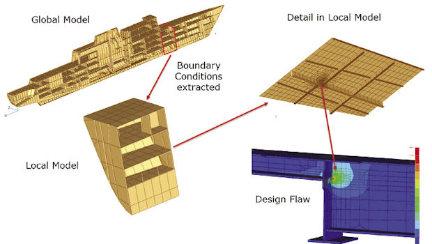
An example is shown in Fig. 6, where a ship model is used as the global model. The objective was to investigate stresses at a design flaw. The load cases analyzed in the global model were used to map the displacement boundary conditions at the global/local interface into the detailed local model. The results of the global model can be considered as a database—from which local region results can be extracted to carry out local checking or redesign.
Both of the previous analyses could also be done using independent local models. Beam forces at each end of the oilrig joint, for example, could be extracted from a global model and applied subsequently to an independent local model. This boundary force approach is useful, as it verifies the loading in the structure. It does mean, however, that we need to use a minimum constraint method to make sure the model is constrained properly to ground. A model in balance must still be properly constrained.
 Fig. 6: A global/local analysis of a ship.
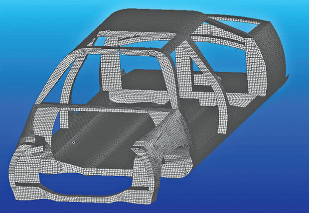 Fig. 7: A full mesh model of a vehicle body in white (BIW).
We also have to be careful when interpolating forces from the global-to-local model across the boundary. With beams, we are dealing with point forces; however, with continuous shell or solid elements, we are dealing with a distribution of forces. We must maintain equilibrium between the models, but must also be careful of inaccurate stiffness representation on the boundary:
- If we model part of the local detailed model with a lower boundary stiffness, the resultant deflections will be higher, and the load path will move away from this region.
- If we allow low stiffness “widgets” (structures that will carry no load in practice) into the boundary region, we may have very large localized displacements.
- Part of the boundary may have a reduced stiffness thanks to the onset of buckling, which is not ideal in the global model. There is then a mismatch in effective stiffness.
If we use the local modeling to investigate design configuration changes, varying damage states, etc., we must avoid changing the overall stiffness assumptions made between the global and the local models. For example, we cannot take a local section out and introduce an elevator shaft through the decks with significantly different stiffness. The boundary conditions mapped from the global model, without the elevator shaft, are now invalid.
Super Element Analysis
The overriding consideration in global/local modeling is that the strain energy on the global and local boundaries should balance. Strictly speaking, we should use both displacement and force at the same time to achieve this. We cannot do this in normal analysis, and have to pick one or the other. However, in static super element analysis, strain energy compatibility is enforced.
The super element method is complex, and its use has tended to be restricted to either experienced analysts or to companies that have invested in incorporating the technique into “black box” procedures. Despite this, it is useful to be aware of the method, as several software vendors have recently started to make the process more usable to the general community.
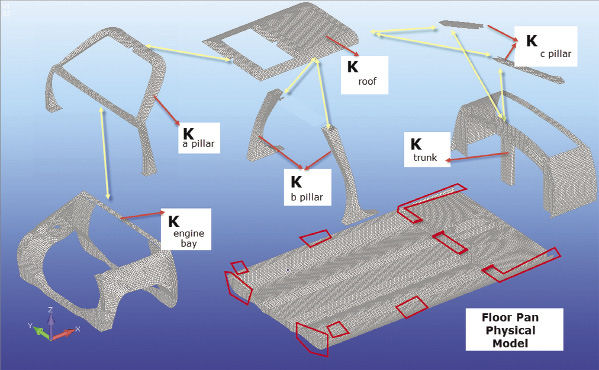 Fig. 8: Components reduced to component stiffnesses, and assembled into the floor pan physical model.
Super element technology allows an engineer to make a FE model of every component of a large system, such as an automotive body in white (BIW). Each component model is translated from its usual, “physical” format of nodes, elements, properties, loads, etc., to a set of structural matrices that represent the same information. Common boundary nodes exist between the components, so that all component matrices can be combined. The complete system can then be solved, and the results passed back to each component.
For example, Fig. 7 shows a full mesh for a vehicle, with no super element reduction. Fig. 8 shows the same vehicle, where the floor pan is used as the base or residual structural model, and super elements are added in as system matrices.
There is coupling defined between the interface boundary nodes on the floor pan and each of the engine bay, A-pillar, B-pillar and trunk components. On each interface, the nodes from each side must occupy the same position in space.
There is further coupling between components—the engine bay and A-pillar, for example. There is also a set of components that are indirectly linked via the first-level components, such as the roof being connected to the floor pan via the A-pillar, B-pillar and C-pillar (the last via the trunk). A wiring diagram is essential to keep track of the overall scheme.
The advantages of the super element approach include the fact that the creator of a component does not need to pass any detailed physical information to the person assembling and running the overall system model. The assembler could easily be restricted to seeing the component stiffness matrix and position of boundary nodes. The component designer, however, can see the full response of his or her model when attached to the system. Confidentiality is maintained both ways if required.
It can be an advantage to reduce model size for advanced analyses like nonlinear and dynamics for both performance and housekeeping. For a large system with many components, it can be convenient to split up a model between parallel project teams. For example, different components may have reached different design maturity—but as long as the interfaces are defined, a full system model can still evolve with the latest component designs.
Cost-Effective and Convenient
The use of global-to-local modeling can keep the cost of analysis down, and convenient in allowing logical breakout of local components. Placing the local model in situ, with only a single run needed, is the most intuitive and straightforward method, as long as care is taken over the global-to-local interface.
Analysis with an independent local model requires accurate and meaningful interpolation of either boundary forces or displacements. Some practice and comparison with high-fidelity benchmark examples will help to give confidence in the method.
The super element approach is the most technically exact method, and should give higher accuracy. However, the choice here largely depends on the ease of use in super element setup and analysis of the FEA software implementation available.
Subscribe to our FREE magazine, FREE email newsletters or both!
Latest News
About the Author
Tony Abbey is a consultant analyst with his own company, FETraining. He also works as training manager for NAFEMS, responsible for developing and implementing training classes, including e-learning classes. Send e-mail about this article to [email protected].
Follow DE

