Moving into the Nonlinear World with FEA

By Tony Abbey

Most engineers traditionally migrated from the linear finite element analysis (FEA) world into the nonlinear world when faced with stress levels above the elastic limit—in other words, plasticity. These days,  it is more likely that components in an assembly make contact when loaded or unloaded, and you need to model that situation. Now you are off down the nonlinear path!

I had a colleague who steadfastly declared, “The world is nonlinear.” He was quite right, but we would much prefer when doing FEA to keep things as simple as possible and ignore that fact. A lot of the time we can get away with this, but sometimes we can’t.

After a quick dabble in nonlinear FEA, a lot of engineers understand the reason for the coyness: Nonlinear analysis is tough to do effectively and efficiently —it is a steep learning curve.

The Nonlinear Strategy

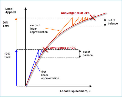
When we carry out a nonlinear analysis, we are taking a journey into the unknown. Fig. 1 shows a typical nonlinear history. Notice how the load is now broken down into smaller steps. We can’t just apply the total and hope we get a good result. We have to tiptoe up the load scale.

Here we see two load increments: up to 10% and up to 20%. In practice, these may be as low as 1% increments for a highly nonlinear problem.

At each load increment, the solver has to iterate within the solution to find a load balance. The first approximation is a linear analysis,  so it will not be in balance if the response is nonlinear. The solver transforms the solution into a one-dimensional search path, looking for this balance point.

Fig. 1: Nonlinear strategy.

Once the first balance point is found, we have the first known point in our journey. We can then carry out another exploratory linear analysis and see where that takes us. Again, it is an approximation and we have to iterate to find the nonlinear balance point. The journey continues, finding each balance point up to the full 100% loading. We have then established the nonlinear response at each point in the structure.

The cost of doing these successive iterations can be quite significant. If it takes 10 steps, with each one needing a full stiffness matrix update and solution, that means the analysis is 10 times more expensive than an equivalent-sized static solution. There are many strategies to make this updating as parsimonious as possible, so it is not quite so savage a scaling effect on cost. But for a highly nonlinear structure, there is often no other option than to accept the cost.

The convergence to a balance at each step can be the cause of much heartache. If we use too large a step, or have highly nonlinear events such as large contact changes, big changes in the material slope or abrupt collapse due to nonlinear buckling or snap-through, the solver can have a tough time seeking a balance. We may even find that there is no physically realizable solution—as in the case with a collapse load.

This leads us to one of the most important tips: Simplify the nonlinearity as much as possible. If you have contact, friction, geometric nonlinearity and plasticity all going on at once, take a step backward and introduce these effects one at a time. You may “bond” the contact surfaces together for simplicity, and make the material linear. Now you can shake down the geometric nonlinearity and get that to work. Even here, you may want to start with a simpler model to establish the physics of the structural behavior and work up from there.

Material Nonlinearity

When the stress level in a component exceeds the yield point, the material in the affected zone starts to go plastic. The presence of plasticity means the material is following a nonlinear stress strain curve,  typified by test results shown in Fig. 2. Some materials show a distinct transition from linear elastic to nonlinear plastic at a clearly defined yield point; others show a slow drift off the linear curve. Fig. 3 shows how to deal with the “drift”—an arbitrary line at 0.1% or 0.2% strain is drawn parallel to the initial slope, and the yield point is taken to be where this crosses the material curve.

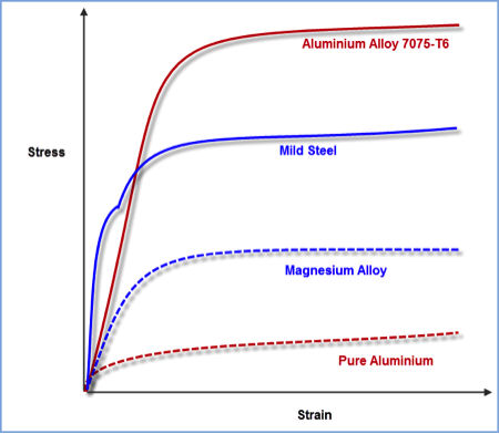Fig. 2: Various metal stress-strain curves.

We usually have to simplify the actual stress strain curve in an FEA material model. The input to FEA can be rationalized by an elastic linear section, whose slope matches the linear material stiffness E, and a plastic nonlinear part, which can be a constant slope (the two slopes are described as a bilinear fit), or a varying slope defined by a data table. Both types are shown in Fig. 3.

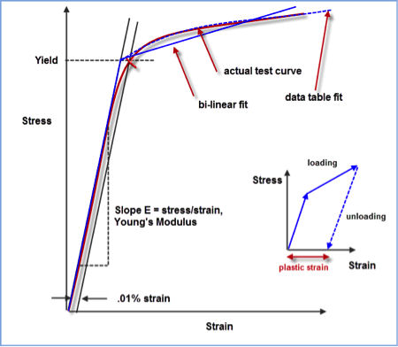Fig. 3: FEA material fit to data.

The Fig. 3 inset shows the loading and unloading along the elastic and plastic curves. The unloading occurs parallel to the elastic curve,  and leaves a “locked-in” strain when fully unloaded. This is the residual plastic strain left in the structure, with associated permanent set.

If a nonlinear solution is used, all elements in the model are monitored to check for values above yield. If this occurs, the elements in the affected regions have a modified material stiffness term invoked, which uses the new slope of the elastic plastic curve.

In general, we need to tiptoe along this curve so that stiffness updates are carried out slowly, and equilibrium enforced as we go.

Fig. 4: Progressive axial stress distribution.

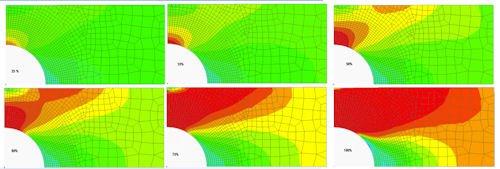
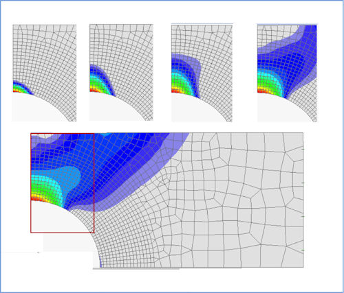
If we adopt this gradual-increment approach, we can capture the growth of a plastic zone. It is important to realize, however, that as the plastic zone grows, the stress flow in the component and around the plastic zone will change. Often, a plastic “lobe” type shape appears, and then grows. Fig. 4 shows a sequence yield stress front growth around a hole in a plate as load is increased. Fig. 5 shows the corresponding plastic strain growth.

Fig. 5: Progressive plastic strains.

We may have a situation where only very local plasticity is seen, such as at a local notch or other stress raiser, or at the extreme fiber positions of a beam in bending. The analysis tends to be stable as the overall stiffness changes are small. Conversely, as the plastic zones spread, such as in the final stages of the loaded hole in Fig. 5, large sections of the model are affected and the overall stiffness changes can be significant. This makes it difficult for the nonlinear solver to handle the solution.

Geometric Nonlinearity

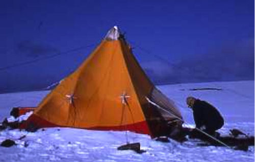
Looking at the tent in Fig. 6, we can see the walls have been deflected inward under the wind pressure. Internal balancing loads in the tent wall develop as it moves into this shape, and the corresponding internal stresses are dominated by membrane—or in-plane stresses. It wouldn’t make sense to think of the tent in its undeformed, flat, initial state, trying to resist the wind pressure. When a structure has to deform and the loads can only be balanced in that configuration, the phenomena is called geometric nonlinearity. Notice there is no material nonlinearity here—it is all down to the loading and deflection.

Fig. 6: Nonlinear deflections.

Contrast this with a stiff bridge deck, carrying its own weight plus traffic, wind loading, etc. The loads will be “beamed” from the bridge deck to the foundation structure, with very little deformation of the bridge deck. We can ignore the influence of deformations to get a load balance;  this is a linear solution. Many years ago, I had a client who tried to analyze a tent wall with a linear solution. It can’t work because it needs to deflect to transmit the loads.

Often in practice, we get to a “middle ground” when we come to deflections of thin-walled structures, like plates. The linear theory we use in FEA assumes the deflections normal to the plate are, at most, around 25% to 50% of the plate thickness. Under that assumption, pressure load is “beamed”  from the center to the edges, like the bridge. If deflection goes beyond this,  the load transfer starts to pick up the tent-like membrane or in-plane loading. The stress system changes from all bending and shear to bending, shear and membrane. We need to move to a non-linear FEA to pick this up.

We can see the geometric nonlinear term coming into play in a simple example. Fig. 7 shows a rigid bar connected to a pivot at one end. A linear rotational spring resists motion at that end. We apply a small force at the free end of the bar, and it rotates slightly about the pivot. The movement applied to the bar balances the torque produced in the rotary spring. The bar movement (force times length) equals the torque reaction in the spring. We can also estimate the rotation of the bar about the pivot by knowing the torque and the spring rate.

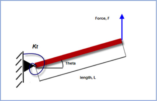Fig. 7: Rigid rod and torsional spring.

The important point here is that we carry out the force balance in the undeformed position as a linear approximation. This is the basis of linear analysis.

As the bar rotates, the movement gets smaller, because the line of action of the force creeps closer to the pivot. If we include this effect, we are balancing the rod and spring in the deformed position. This is a nonlinear solution.

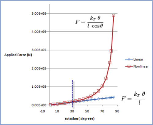
The linear solution ... just stays linear! It doesn’t care how absurd the solution gets. Think about a force of 2E5 N applied at the tip. The rotation is “off the clock.” We could extrapolate and calculate a rotation that implies the rod does four or five complete pirouettes around the pivot. It is an absurd answer, but we often see exactly that in a linear analysis that is trying to handle nonlinear geometric response. We can’t map this back to a physically meaningful situation. We have overshot the limits of a linear analysis, and need to move to nonlinear analysis.

The nonlinear solution shows a divergence away from the linear at around 30 ° of rotation. If we apply 2E5N now, we get a rotation of around 82 ° —clearly balanced only in a nearly vertical deformed state.

Sometimes, analysis with geometric nonlinearity is called a “large displacement” analysis. I don’t like this term because it begs the question “how large is large?” Every analysis is material-, loading- and configuration-dependent, so there is no real answer.

Geometric Nonlinear Load Types

The pressure force in a tent wall will always “follow” the tent wall deformation. An inflating toy balloon changes shape dramatically, but pressure is always normal to the surface. The rod force was applied and stayed in the vertical sense, whatever the rod rotation. This is a non-follower load.

It is important to establish what type of loading is present. Gravity loads will always be non-follower, but a bearing load from an adjacent structure can be either.

The setup of a follower force is straightforward if it is pressure-loading. All FEA solvers should be able to automatically adjust the normal direction under deformation.

A load applied as a point force is trickier. The vector associated with the force direction has to be updated. Typically, a set of “anchor” nodes is used. As these deform, they will update the force vector. However, if nodes are badly chosen, the force vector is slaved to these and can result in bizarre changes. It is better to convert any point forces to a pressure distributed over a small “pad” of surface area. This is good practice,  even in a linear analysis, to avoid spurious localized stresses.

Contact Implementation

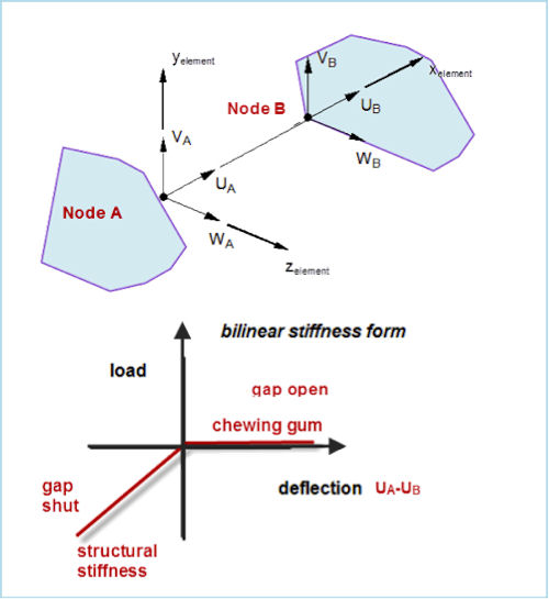
The early implementations of contact were nothing more than a set of nonlinear springs, as shown in Fig. 8. These were referred to as gap elements. They are little used these days, but illustrate some of the principles still used. When the gap is open, the spring stiffness is weak, like chewing gum. When the gap is shut, the stiffness is the same as the surrounding material.

Fig. 8: Original gap element.

To create a “closed gap,” the nodes A and B must pass through one another. This creates a problem in that we are not now modeling the real situation, both nodes just touching and then moving together. Only by having penetration can we get a resisting force. This is basically the penalty stiffness method used in many contact algorithms.

To model reality, it is really required to make contacts be just touching, and develop the corresponding reaction forces in a more natural way. This is done by an auxiliary set of forces introduced to make the contact and form the reaction forces. This method is known as the Lagrangian method,  and is a later development.

Many solvers actually use a mix of these two methods. The search for good stable methods still continues, and we can expect new solver developments over the next few years.

The technology has moved beyond simple gaps and now covers whole regions of contact mesh. Now arbitrary zones of a model can be assessed to see whether they will move into contact or separate as the loading is applied. The terminology of a “master” surface and “slave” surface is often used to differentiate the two surfaces that come into contact. A typical setup is shown in Fig. 9. In single-sided contact, the regions formed by the master elements search for slave nodes that will pass through the net and will form connections. The region can be shell elements or the faces of solid elements.

Fig. 9: General surface contact.

The computational cost of this search can be quite high—rather like ray tracing, so methods are used to cut down “who sees whom”  in a general solution. Cost equates to solution time and memory requirements. Still, techniques are getting more efficient as technology improves, so we can expect to see the cost going down and versatility increasing. One example is that double-sided contact where slave surfaces look for master nodes is now very common.

Controlling Jaggies

Other issues include getting rid of the “jaggies.” The FEA mesh is usually a discontinuous discretization, and the slave region introduces into master regions, as shown in Fig. 10. This results in a set of artificial point loads, which destroy the attempt to have continuous bearing forces, for example. This is very difficult to avoid, even by careful meshing.

Fig. 10: Avoiding the “jaggies.”

Techniques are available that fit a common interpolated surface to which the nodes move, or even inherit the actual CAD geometry surface. A smooth bearing load distribution can then be achieved.

Another common issue with contacts is that of “loose”  components not properly abutting each other. A typical CAD model will place components at nominal positions—for example, a pin and lug defined concentrically. In FEA, we require the pin to start off being in bearing contact with the lug to establish a load path. If we can modify the CAD model, that’s a great help. However, it can be difficult to establish a stable initial load path at small initial load steps.

Other methods include putting in very weak springs to help stabilize—or in an extreme case, running a time-based analysis. The time scale does not matter, but what really helps is that each new load step convergence is not just working with an updated stiffness; we are passing forward the dynamic effects —and the key here is inertia.

There are many types of nonlinearity; we have looked at the main areas. It is important to assess what level of nonlinearity is needed to adequately model the problem, then take small bites of the cherry and explore the nature of the nonlinearity carefully. We want to start simply and explore—and far we need to go!

Tony Abbey is a consultant analyst with his own company, FETraining. He also works as training manager for NAFEMS, responsible for developing and implementing training classes, including a wide range of e-learning classes. Send e-mail about this article to [email protected].

MORE INFO

FETraining

  NAFEMS