
FIG 2: Mesh detail in latch and key nodes.


Latest News
January 1, 2015
Editor’s Note: Tony Abbey teaches live NAFEMS FEA classes in the US, Europe and Asia. He also teaches NAFEMS e-learning classes globally. Contact [email protected] for details.
One of the most difficult aspects of setting up an FEA (finite element analysis) model to simulate the real world is applying realistic boundary conditions. This means understanding how the structure is loaded by external forces and how it is constrained from moving globally in space. Sometimes the distinction between whether a structure should be fixed to the ground or loaded externally can become a little blurred. It is up to the analyst to decide how to deal with this.
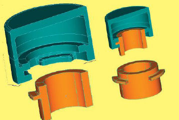 FIG 1: Two part assembly showing contacting latches.
An example structure is shown in Fig. 1. It is a two-part assembly. The top fitting latches onto the lower fitting using a bayonet type connection, by pushing down and rotating through 60 degrees. A seal runs around the entire mating face, but is not shown here. The bayonet connection leaves three pairs of latches in contact under an internal pressure loading. The assembly has a plane of symmetry, and this is used to advantage in the FEA model, as shown in the figure. The run time is reduced by a factor of four with a half model.
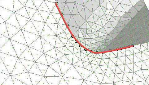 FIG 2: Mesh detail in latch and key nodes.
A typical latch mesh is shown in Fig. 2. On the top fitting, there is a stress concentration at the inner fillet radius and this is the subject of investigation. The line of nodes used to check the stresses is shown in the inset in Fig. 2.
Checking Stress Levels
If a linear static analysis is used initially to check stress levels then there are three ways of doing this. Fig. 3 shows how the latch can be loaded and the top fitting assumed held remotely (3a), the latch can be clamped by a constraint to ground and the load applied to the top fitting remotely (3b), or a glued contact can be used to join the latch and mating inner component (3c).
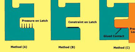 FIG 3: Latch loading and constraint methods.
The motivation for making these linear assumptions about the bearing loading path and associated stress distribution is that a linear analysis will usually be much faster and easier to run. There is always a risk in running a non-linear analysis in that convergence is never guaranteed and may be difficult to achieve. A ‘quick-look’ equivalent linear analysis is always worth trying.
Applying equivalent pressure to the latch face as in Fig. 3a is considered a “soft” loading. The idealization provides no stiffening, however an assumption has to be made about the pressure footprint. Here it is assumed to be evenly distributed right up to the edge of the latch contacting faces. The result is shown in Fig. 4a and is a classical stress concentration distribution. The mesh density is adequate as shown by a separate mesh convergence study.
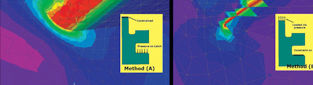 FIG 4: Stress contours for pressure and constraint.
Traditionally, clamping the latch as in Fig. 3b is considered a “hard” load path. The idealization represents a latch face that is bonded to an infinitely stiff mating surface. At the edge of any constraint run out like this a stress singularity is created. The FEA model assumes a jump from infinitely stiff to flexible over a single element width. This is like an extreme example of a stiff material ‘digging in’ at its edges into a soft material. The line of high stresses, representing the singularity, is shown in Fig. 4b. However, what is surprising here is that the stiffening effect of the constraint does reduce the level of the stress concentration compared to a “soft” pressure distribution as shown in Fig. 4a. The stress plot around the fillet is shown in figure 5 for both soft pressure, hard clamping and also glued contact.
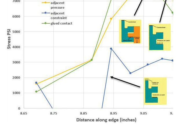 FIG 5: Stress variation around fillet for cases 3a, 3b, 3c.
The soft pressure distribution (3a) and glued contact (3c) give very similar stress distribution results. There are two idealization observations here: the pressure footprint for the glued contact is similar to the soft pressure. The stiffening effect of the inner glued latch does not seem to affect the stress distribution significantly. The singularity caused by the harsh constraint (3b) is shown in Fig. 5 and dominates the result. The constraint also seems to reduce the stress concentration significantly, presumably by altering the effective load path to be more favorable to the fillet region.
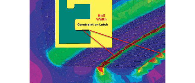 FIG 6: Attempting to move the constraint edge singularity away from the fillet.
It seems that the constrained method is a poor idealization for this geometry; it gives a spurious singularity, which is adjacent to the fillet radius and is effecting the distribution. There is also a slight tendency for the glued contact to give a spurious stress raiser at the edge of the contact. A contact run out is often a source of mild singularity. Similarly, the general contact method (in a subsequent nonlinear analysis) also gave a slight stress raiser at the contact edge, and also a reduction in peak stress distribution over the soft pressure. A soft pressure distribution is therefore recommended. This may be surprising, as a general contact surface model would traditionally be assumed to be the most realistic idealization. However, it shares the tendency of glued contact to give a spurious edge effect and there may be concerns that this affects the peak stress.
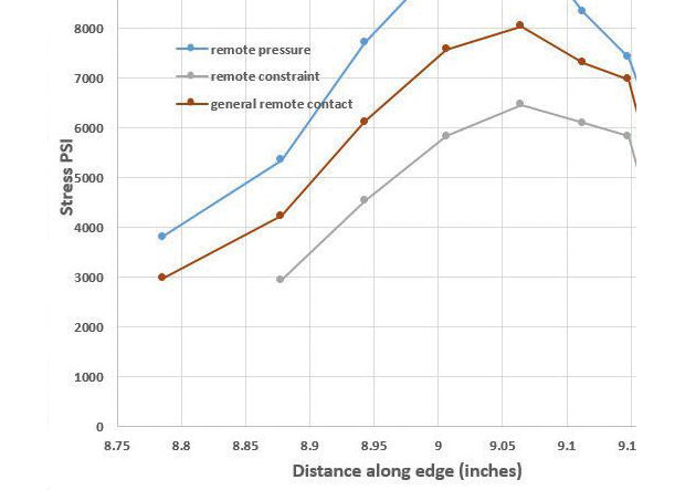 FIG 7: Distribution of stress, offset contact region assumed.
An alternative approach to method 3b is to apply the constraint with a separation from the fillet edge. The line of singularity is now moved away from the fillet toe to the new latch mating edge. This leaves the fillet radius freer to develop a reasonable stress distribution. The region of stress singularity is still present, but is now away from the fillet radius, as shown in Fig. 6. To compare the peak stress value, it is necessary to run a similar pressure distribution footprint. A new general contact analysis result is also compared. The three new methods are shown in Fig. 7, with a graph of the stress distribution.
Fig. 7 shows that the singularity is moved away from the fillet toe in the constraint method and the general contact method. However, as before, the constraint method is over constraining the latch feature and so the fillet region does not develop the full peak stress value. The contact method also appears to constrain the solution compared to the “free” pressure loading method. The stress has increased in all cases due to the bigger offset of the line of action.Offsetting the contact footprint would be a reasonable approach because in hand stress calculations we would always assume the line of action was conservatively offset, rather than through the mid line of the latch. The actual bearing contact footprint is really an unknown in many situations. Without some test evidence it is difficult to assess if the general contact surface method gives an accurate representation. In this particular case, the offset moment is the dominant factor in the peak stress at the fillet radius and it is therefore important that a conservative approach is taken.
Don’t Be Misled
The “hard” constraint method of applying a boundary condition is seen to be misleading in this case for two reasons:
1. The edge of the constraint is a singularity and influences the fillet toe directly by giving unrealistic local stresses.
2. The constraint over-stiffens the latch flange and reduces the peak stress from that expected by cantilever action of the latch flange.
The general contact and glued contact methods rely on a realistic bearing footprint, hence load line action. The peak stresses seen in the fillet are reduced from the equivalent ‘free’ pressure distribution, suggesting that the line of load action is closer to the fillet toe in these methods. Without test evidence, it is difficult to assess whether this conservatism is warranted.
Hand calculations, based on bending stresses at the weld toe (distance 8.88 in.), with assumed stress concentration factor at this position, show stresses at this point are close to the indicated stresses. However the peak stress is at a distance of 9.06 in., the center of the fillet in all cases.
In summary a “free” equivalent pressure distribution with a conservatively assumed line of loading action is probably the safest assumption to make in this case.
| Method | Label | Peak P1 Stress |
| Overall Press | 3A | 8020.539 |
| Adjacent Constraint | 3B | 3214.853 |
| Glued Contact | 3C | 7396.921 |
| General Contact | 7432.468 | |
| Peak stress values at fillet. | ||
In my next article, we will discuss how to apply equivalent pressure distributions throughout a structure to achieve balance, avoid any direct constraint boundary modeling, and rigid body motion.
Subscribe to our FREE magazine, FREE email newsletters or both!
Latest News
About the Author
Tony Abbey is a consultant analyst with his own company, FETraining. He also works as training manager for NAFEMS, responsible for developing and implementing training classes, including e-learning classes. Send e-mail about this article to [email protected].
Follow DE

