SOLIDWORKS Simulation Overview, Part 2
Pre-processing and Meshing News
Pre-processing and Meshing Resources

Dassault Systemes
July 1, 2018
In part one of this SOLIDWORKS Simulation overview, we looked at the aircraft keel section shown in Fig. 1 and focused on the meshing task. In part two we will be applying loads and boundary conditions, running the analysis and post-processing the results. Fig. 1 also shows the loads and boundary conditions. The boundary conditions consist of two components:
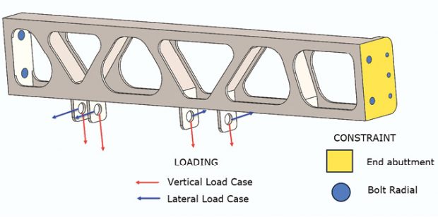
1. end abutment faces, which prevent the keel section moving fore and aft at both ends, lateral and vertical degrees of freedom (DOF) are free; and
2. longitudinal bolts, which are assumed to be acting in shear to restrain vertical and lateral motion.
Fig. 2 shows the setup of the constraints within SOLIDWORKS. Notice that SOLIDWORKS describes constraints as “Fixtures.”
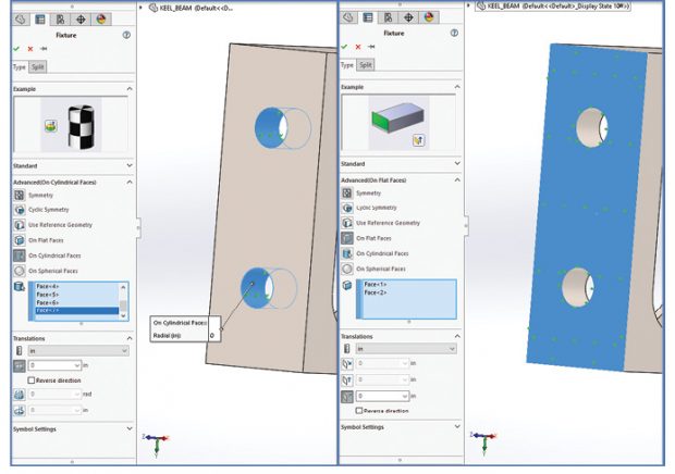
The left-hand image in Fig. 2 shows the bolts being constrained. The Roller/Slider fixture type is chosen and then the Advanced option is selected. This has an option to constrain on cylindrical surfaces. In this case I have chosen to constrain the radial direction. The axial and circumferential directions are free. This assumes that the bolt will act in shear, by taking bearing loads on the bolt shank. The local stresses won’t be accurate, because as well as compression on the bearing face, there will be tension on the back face. For the overall model assessment this assumption is reasonable. All the bolt regions shown in Fig. 1 have been treated this way.
The right-hand image in Fig. 2 shows how the abutment faces were simulated. The assumption here is that compressive bearing load is carried across both abutment faces. Any prying effect that would tend to gap at the top edges under bending is ignored. This is something to check in the stress results to make sure that there isn’t significant tension that may be trying to unrealistically pull against the abutment face. Both end abutments are shown in Fig. 1.
Two load cases are considered: A vertical load case with a distribution of downward forces in the lugs and the horizontal load case with the distribution of lateral forces in the lugs.
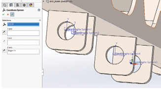
Fig. 3 shows the preparation work needed to set up bearing loads at each lug. We need a center point that can be used to define a coordinate system for each lug. The objective is to have the Z axis aligned as the center of the bearing distribution. The creation of this supplementary geometry is straightforward and can be done within the Analysis Preparation tab of the command manager. This means we can stay within the simulation environment.
The menu in Fig. 3 shows the “pinned” menu option highlighted underneath the Coordinate System header. This is a feature common throughout SOLIDWORKS and means that the menu is kept in place but refreshed for each successive coordinate system creation. This speeds up the workflow.
Once the local coordinate systems are set up, the bearing loads can be applied, as shown in Fig. 4.
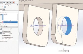
The menu in Fig. 4 shows a bearing face being selected and a vertical direction being picked. The load distribution is assumed to be a sinusoidal distribution over 180°. The selection is limited to either vertical (x) or lateral (y) directions, positive or negative. Oblique angles of loading will require a coordinate system orientated in that direction.
The feature tree shows eight instances of lug loading, split between each of the two load cases.
Load Case Manager
The intention is to investigate each of the load cases separately, to identify the individual responses and then to investigate the combined load case. This is a standard practice in many industries, and it’s one that I highly recommend. There are two ways to carry this out in SOLIDWORKS. The conventional approach sets up a simulation study for the two individual load cases and one for the combined load case. This requires three analysis runs from within each simulation study. But it means the full post-processing capabilities are available for each result set.
The alternative is to use the Load Case Manager, found by right mouse-clicking on the main analysis icon in the feature tree. This will allow a single analysis run, within a single study, to include many load cases. For versions 2018 onward, full manipulation of the results entities is available. Prior to version 2018 there is limited capability for post-processing, and I would not recommend its usage.
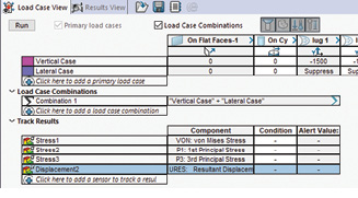
Fig. 5 shows the load case manager. In Fig. 5, using the Load Case Manager, I have labeled the two load cases as vertical and lateral. The appropriate constraints and loads are then selected or suppressed as shown in the spreadsheet.
The combination case is created automatically by spawning a default equation within SOLIDWORKS. This is 1.0 times the vertical case added to 1.0 times the lateral case. These scale factors can easily be overwritten.
The next block in the spreadsheet defines the result quantities to be post-processed. These will spawn instances of contour plots for each of the stress types indicated and for the displacement.
If you are using the Load Case Manager, then the analysis runs from this spreadsheet by clicking on the Run button. If you are not using the Load Case Manager, then each run is launched in turn within the appropriate simulation study.
The Results
If the studies are run independently then a typical feature tree shows the instances of results visualization. They control by default; von Mises stress, maximum and minimum Principal stresses and X Direction stress. Right mouse-clicking on the stress object allows manipulation via three Property Manager dialogue boxes. The result quantity can be changed, nodal or elemental values can be selected, and maximum and minimum values in the contour plot can be set; there are even further options. This versatility allows for a powerful post-processing tool.
If the Load Case Manager is used then the controller is slightly different. The default results are no longer available from the feature tree. Instead, under Load Case Results, the stress or displacement plot type can be selected. The load case is also selected and highlighted in the spreadsheet. By synchronizing the stress or displacement plot type with the load case, then any result quantity can be seen. A summary table reporting stress or displacement quantities for each load case can be defined by the user as the maximum value or a variety of other filters.
The advantage of the load case manager in this context is that there is no need to switch between simulation studies.
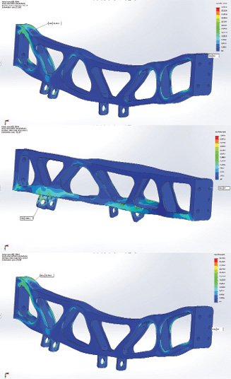
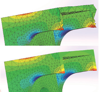
Fig. 6: One Mises stress distribution for (top) vertical case, (center) lateral case, (bottom) combined case.
Fig. 6 shows the von Mises stress distribution for the vertical, lateral and combined cases. The peak stresses seen in each case are 38459 PSI, 3800 PSI and 39185 PSI. The vertical case clearly dominates; however, it is always worth investigating contributing cases to see if there are any critical local effects.
In fact, the local lug stresses are not meaningful in the combined case. Two independent sine-bearing load distributions are being incorrectly combined. A separate load case would be required with a single sine distribution about the correct resultant line of load action. However, the overall peak stresses are away from this region. A local lug model would probably be sufficient to demonstrate this point.
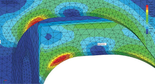
The peak stresses in local regions are investigated further, for the combined case, as shown in Fig. 7. The left-hand end upper fillet radii are the critical regions.
In a previous series of articles, (DE March, May and July 2016) I looked at various ways to assess stress distribution. We use von Mises stress to attract our attention to the peak stress regions; however, the distribution shown in Fig. 7 is typical in that we don’t know what type of stress is being developed, and we have no understanding of the load path based on that plot alone.
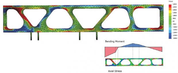
It is easy to switch component stresses within SOLIDWORKS, and in Fig. 8, I have used the axial or X Direction stress.
I have deliberately set the upper and lower bound on the stress contours to a low magnitude of +/- 3000 PSI. This is easily done with the SOLIDWORKS post-processing controls. The point of the exercise is to understand how the stress flows axially through the structure. I’ve also shown an inset of a traditional Bending Moment diagram for this distribution of forces and built-in ends. The moment distribution confirms the presence of direct bending stresses at the top and bottom surfaces of the keel beam. The switch-in sign from the end regions to the center regions is clearly seen. The stress concentrations overlaid over the basic beam stress distribution can also be identified. This is a qualitative assessment, but it does allow an understanding of how and why these axial stresses are present. The fillet pair identified in Fig. 7 can now be understood further. The left-hand fillet is in a state of compression, while the right-hand is a state of tension. This is an important distinction; tension may indicate fatigue problems, and compression may indicate local crippling problems.
Two further useful tools within SOLIDWORKS post-processing are shown in Fig. 9.
Fig. 9 shows two forms of section cut. The lower is an arbitrary cut, controlled by slider bar or user input. It gives an excellent sense of the stress distribution through the depth and again confirms the local bending sense. However, the results are interpolated within elements at the arbitrary cut plane. A useful adjunct to this is the element edge plot, which preserves the true face of the elements in that cut zone. This gives a true sense for the quality of the elements and hence the stress distribution through the cut region.
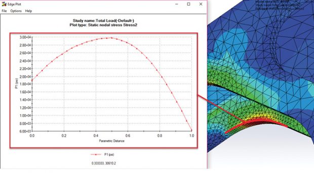
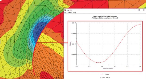
I always consider contour plots to be subjective and look to graphs of stress versus distance for a more definitive understanding. Figs. 10 and 11 show such graphs.
Taken together, the contour plots and graphs shown in Figs. 10 and 11 give an excellent understanding of the stress variation running around the inside of the fillets. These results, and the axial stress results shown in Fig. 9, uncover the full meaning of the von Mises stress distribution shown in Fig. 7.
The graphs shown in Figs. 10 and 11 are easy to produce, using a Probe tool. Any geometric entity, in this case the edge curves, can be selected and used as the basis for the graph. The data can also be exported as a CSV file, ready for further manipulation.
Conclusions
SOLIDWORKS simulation has a rich set of tools for analysis definition, meshing, loads and boundary conditions and post-processing. The user interfaces are straightforward to use, particularly if using the defaults. Because of this, there may be a tendency to stay with these. However, by exploring the deeper menu options and functionality, a user can develop more sophisticated analysis techniques. This does take some determination and patience, but can be quite rewarding.
More Dassault Systemes Coverage

For More Info
Subscribe to our FREE magazine, FREE email newsletters or both!
About the Author
Tony Abbey is a consultant analyst with his own company, FETraining. He also works as training manager for NAFEMS, responsible for developing and implementing training classes, including e-learning classes. Send e-mail about this article to [email protected].
Follow DE

