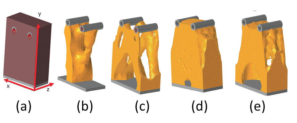
Fig. 1: (a) design space, (b) axial load, (c) bending load, (d) torsional load and (e) combined loads.


Latest News
October 1, 2017
Robust Design Under Loading
Fig. 1(a) shows a design space ready for topology optimization. The constraint is applied as a fixed constraint across the base of the gray-colored object. Loading is applied to the inside face of the two gray-colored cylinders at the top of the object. The design space is shown in brown. The non-design space, embracing the load and constraint regions, is shown in gray. Preserving the regions where constraints or loading is applied is an important aspect of topology optimization. Commercial topology optimizers have different behaviors, but in general, the developing topology configuration will be very unpredictable if the loaded surface or the constraint surface can be eroded during the element deletion process. A situation could arise where the whole structure is disconnected from any loading or constraint path. As that condition is approached, the solution becomes nonsensical.
 Fig. 1: (a) design space, (b) axial load, (c) bending load, (d) torsional load and (e) combined loads.
The two cylinders are first loaded in the vertical (Y) direction. However, the loads are not equal, so we will anticipate a different load path created under the two load application points.
Fig. 1(b) shows the resultant topology configuration found by keeping 25% of the original volume as a target and minimizing the compliance. The dominant load path is clearly seen on the left side of the structure. The overall load path has migrated to the left. The ability of the reaction zone, defined by the constraints remaining, to adapt in this way is an important characteristic of the topology optimizer. The most efficient load path can develop, and inefficient material be deleted, if the constraint distribution can change.
In Fig. 1(c) the topology optimization is rerun, this time with a load in the lateral (-X) direction, resulting in a bending moment about the base. The configuration has changed dramatically. The constraint has now migrated to the extreme ±X axis positions. This will clearly maximize the bending stiffness. Ligaments are formed, connecting each of the four extreme support positions to the loaded cylinders.
In Fig. 1(d) the two cylinders are loaded axially, one in positive Z and one in negative Z directions. This gives the component a torsional loading. The distribution of material is a logical solution as it increases the torsional stiffness most efficiently. The material is spread out as far as possible toward the boundaries of the design domain. It is a thin-walled box section, and the wall thickness is almost certainly governed by the minimum member size that can be achieved by the topology optimizer, consistently throughout the structure. In practice, we need to guide the optimizer here by providing a cylindrical design space, rather than box-shaped space. At the loaded cylinders, a perfect hollow box shape is not possible. This is a typical situation where we are forcing the topology optimizer down a particular route because of our choice of loading configuration. If the torsional input were the only load input, it would make sense to have distributed loading around the periphery of the structure.
So, the implication of the three independent loading actions is clear, three very different structural configurations will be developed. Each of the configurations is the most efficient distribution of material to provide the maximum stiffness. For a robust structure that sees a range of loadings, it is important that the topology optimizer considers all load cases. The load cases are not combined into a single case; each is evaluated separately as shown. The optimizer uses the independent responses of all cases. Fig. 1(e) shows the distribution of material if all three cases are applied.
The configuration in Fig. 1(e) is a compromise across the three independent solutions. The torsional requirement and the bending requirement have been combined to give well-dispersed material at the base, but the constant thickness, thin-walled solution has been abandoned. This illustrates how important it is to make sure that we’ve considered all the cases in a topology optimization study. If we miss a load case, then the structure is almost certainly doomed to fail because it has been designed to avoid that load case. It would just be a matter of luck if other load cases developed an adequate load path that would sustain the missing load case.
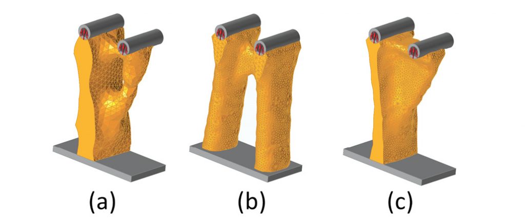 Fig. 2: (a) axial load free form, (b) axial load YZ symmetry and (c) axial load XY symmetry.
One way to improve the robustness of a topology configuration, in the sense of its ability to resist the cases we may miss, is to use symmetry. Fig. 2(a) shows the structure with axial loading applied as before. Fig. 2(b) shows the result with a topology symmetry plane enforced about the central YZ plane.
The bias shown in the configuration in Fig. 2(a) has been removed. This will be a less efficient solution than in Fig. 2(a) because the less dominant load path now has superfluous material. However, if the loading was reversed and the load paths switched, this configuration would be capable of handling the scenario. In many situations, load cases are symmetric, and this is an easy way to create structures that can handle that. I remember doing a detailed stress analysis of an aircraft wing lug during my first few months in the industry. It struck me that the load paths were not symmetric, and I painstakingly designed a configuration that would match the loading. The designers were not impressed, and they gave me many reasons why a non-symmetric lug would be a disaster. This included uncertainty of loading, manufacturability and ease of assembly!
The way that the topology symmetry is defined in the topology optimizer is by simply defining a symmetry plane in YZ and ensuring that the design space is meshed symmetrically. Every element in the original design domain on one side of that symmetry plane is linked to its cousin in the opposite plane. These become a set of constraints, or design variable linking, which effectively slave the two elements together. If one element is deleted, both are deleted and vice versa.
Notice that the loading and constraints do not have to be symmetric for topology symmetry. This is different from normal structural planar symmetry, where all aspects of the loading, constraints and geometry have to be symmetric.
Fig. 2(c) shows a situation with axial loading, and central XY plane symmetry. The result is a more regular dispersion of material, compared with the free form of Fig. 2(a). The loading is still non-symmetric, but the look and feel of the configuration is much more traditional in Fig. 2(c), than in Fig. 2(a). We can imagine this structure being worked up into a quite conventional-looking pillar and bracket. There may be formal reasons why we want to impose the XY or YZ symmetry, which we will cover in the next section, but it’s interesting to see how pushing and pulling symmetry conditions can give us configurations that are perhaps more appealing in an intuitive sense.
Manufacturing Constraints
As I mentioned earlier, in relating my own design experience, symmetry may be required for manufacturing. Most topology optimizers also allow specific manufacturing constraints to be applied. In Figs. 3(a) through (c), an extrusion constraint has been applied in the Y direction and the three combined load cases are repeated. The topology optimizer can now only add or remove elements independently in the XZ plane, as shown in Fig. 3(c). The distribution is then projected along the y-axis. The non-design loading and constraint regions are not extrudable, but the rest of the design region is. Again, in practice it would make more sense to tailor the non-design loading and constraint regions to suit the extruded design philosophy.
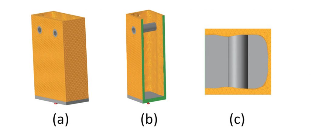 Fig. 3: (a) combined load with extrusion constraint, (b) split view and (c) section view.
Variations on the extrusion constraint include draw constraints, which can be single or double sided. This forces the topology optimizer to create shapes that can be drawn out of single-sided or double-sided molds or dies.
Further extensions to manufacturability include pattern regions. For example, we could have divided our initial design space into three regions by slicing twice in the XZ plane. Each one of these three regions could then be forced to develop a similar pattern. The pattern is arbitrary, but it is repeated as each of the three sets of corresponding elements across the three regions is slaved together. If an element is deleted from one region, it must be deleted from all. Conversely, if it is added in one region it must be added to all. Because the patterning is working on topology, it is possible to have varying sizes of the pattern regions. For example, in a tapered wing rib, the same pattern could exist across different bays, but could be scaled and warped. The topology is identical, but the dimensions have morphed to suit.
Manufacturing constraints attempt to control the “wild child” of topology optimization to produce more realizable structural forms. In most topology-led design evolutions, however, there will probably be a point at which it is more useful to transition to shape or sizing optimization, or think about the structure from a common-sense design perspective. In many ways, the whole point of topology optimization is to explore free-form designs and over-constraining can become unproductive.
In future articles in this series, we will look at case studies using various commercial topology optimizers.
Subscribe to our FREE magazine, FREE email newsletters or both!
Latest News
About the Author
Tony Abbey is a consultant analyst with his own company, FETraining. He also works as training manager for NAFEMS, responsible for developing and implementing training classes, including e-learning classes. Send e-mail about this article to [email protected].
Follow DERelated Topics


