Helping design and engineering professionals discover, evaluate and specify technologies and processes that shorten the design cycle and enable success.
Alert!
Digital Engineering ceased publication on July 1, 2026. This website remains available as an archive of engineering content.
For inquiries or information, please email [email protected].

May 2026 Special Focus: Artificial Intelligence in Design and Simulation
In this Special Focus Issue, learn about the latest developments in the integration of artificial intelligence into engineering workflows.

Design & Simulation Software Guide 2025
In this Special Issue, Digital Engineering presents its second annual guide to design and simulation software vendors.
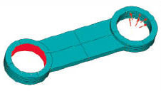 Figure 1: Component loaded and constrained at surface geometry. |
It is a sobering fact that structures can take up an enormous part of an engineer s time in the meshing phase. A complex fabrication may use very little of available CAD geometry when meshing--or worse, be just a 2D drawing image. Meshing can then hit 80% of project time.
For most structures, a good understanding of meshing is important for productivity. Factors include:
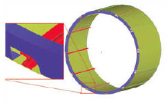 Figure 2: Typical fabricated structure with solid geometry. |
3D Idealization
Idealization defines how we simulate structural characteristics of the component. A component may be defined by CAD solid geometry, having all the information needed to calculate stiffness and strength. The geometry can be "cleaned" to remove irrelevant features such as tooling holes, bolt holes, handles, electronic components, etc. Cutouts and fillets that define detail, but are away from areas of high stress concentration, can be ignored. We apply loading and constraints directly to geometry faces--or edges.
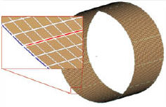 Figure 3: Typical fabricated structure and mesh. |
The geometry has fully defined everything we need (see Fig. 1). We mesh with 3D elements, in a 3D idealization.
Alternatively, we may have a 3D CAD model of a fabrication (such as an aircraft fuselage; see Fig. 2). We cannot mesh with solid elements, because the level of detail implies a model of the order of a billion (1E9) or more elements. The practical performance limit today is around 5 million (5E6) elements!
A fabricated structure requires a 2D/1D idealization strategy (see Fig. 3):
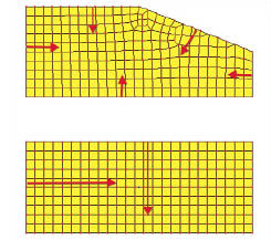 Figure 4: Regular mesh (bottom) and "Pac-Man" type mesh (top). |
Surface geometry is derived, and then meshed with 2D shells and edges with beams or rods. The derivation of the geometry from the original 3D CAD can be labor intensive, however.
The mesh can be created directly without need for parent geometry; this gives greater flexibility in approach.
Quadrilateral (Quad) elements are preferred, and Triangular (Tria) elements avoided, as they have inferior accuracy. A four-sided geometric surface will always generate smooth "mapped" type meshes. An arbitrary five- or greater-sided surface requires an irregular, "Pac-Man-like" generation, by spawning elements from each side and then smoothing confrontation regions where sides meet. Fig. 4 shows surfaces and mesh of the two types.
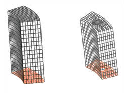 Figure 5: 2.5D meshing, resulting in hex elements. |
Hex and Tet Elements
If a CAD component can be formed by extruding, sweeping or lofting in the CAD model, then we can use 2.5D meshing. A Quad mesh surface forms 3D Brick (Hex) elements by sweeping, or the solid can Hex mesh directly (see Fig. 5). The Hex elements are much more accurate than 3D Tetrahedral (Tet) elements. However, it is difficult to mesh other than in 2.5D or "brick-like" geometry. Many have tried to invent a pure Hex mesher--and so far, none have succeeded.
All 3D geometry can be Hex meshed, given sufficient time and patience. A Rubik s Cube is a good analogy. 3D meshing is a tradeoff--Hex for high accuracy, Tets for speed and ease of meshing. Warning: Do not use four-noded Tet elements. They give appalling results. Only use 10-noded Tets (mid-side nodes present).
Meshing Control
The basic mesh control is global mesh size, applied throughout the geometry (see Fig. 6). Most meshers will calculate this automatically. You can override, but be aware that a reduction from 6mm to 3mm implies eight times more elements.
 Figure 6: Global mesh control. |
Mesh control is improved by defining mesh density at vertices, along curves or on individual surfaces. Curvature-based meshing can be used, because curvature increases and mesh density increases (see Fig. 7).
This hierarchy of controls can be extremely effective, but requires practice. I recommend starting with simple shapes and experimenting with controls to see how they interact (see "Achieving Perfection," page 27).
Checking Mesh Quality
Mesh quality is checked via element geometry such as aspect ratio, value of internal angles, etc. Check documentation definitions, because they do vary across solvers. Contour plots and filters are useful in identifying poor elements. The solver should also give warnings of poor elements. I recommend taking simple geometry and introducing mesh distortions to explore this.
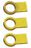 Figure 7: Curvature-based mesh refinement. | 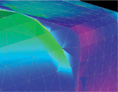 Figure 8: Poor CAD detail, resulting in slivers. |
Simply put, badly shaped elements affect the accuracy of results. In an extreme case, a Tet element can be so distorted that it will "blow up" numerically, causing solver failure. We need to trap this before the analysis starts.
One useful "catchall" check is the Jacobian value. This is based on the mathematics used to evaluate the element stiffness. A good limit value is element- and solver-dependent, thanks to varying mathematics and definitions. I recommend creating a regular mesh, then distorting the mesh and comparing values.
Bad Geometry
CAD geometry can have a variety of problems that directly affect meshing. Small slivers are common at the intersection of curved surfaces, for example (see Fig. 8). The mesh has high aspect ratio Tets in this region, and gives poor results. It is best to simplify or alter the geometry to eliminate the feature, or to add a properly defined fillet.
| Meshing Technique 1. Start with known meshing problem areas. Meshing is always iterative; don t be satisfied with the first attempt. The meshers are designed for fast deletion and remesh. Join up the difficult areas once satisfied. 2. Set a time limit. Time can run away when meshing--it is easy to get diverted by what can be quite a therapeutic pastime! I recommend setting a time limit for specific mesh regions. For example, allot 20 minutes to achieve a best compromise mesh distribution. 3. Focus on the big picture. Keep the overall strategy and element count in mind as you progress through the structure. 4. Do a coarse mesh run to get a feel for stress concentrations, then refine accordingly. Avoid a leap in mesh density, which risks tripping over the performance cliff edge. |
Other CAD features can result in poor meshing, including tolerance errors resulting in "cracks" in the geometry, negative volumes, etc. CAD geometry robustness may be poor because of interdependence of geometric features. Removing a hole or fillet may destroy the integrity of the CAD model.
While this is a big topic, in summary, I recommend a careful assessment of just how "mesh-ready" the CAD geometry is.
Element Stress Accuracy
FEA solves for displacements, not stresses. The displacements are continuous and smooth if the mesh is reasonably fine. The derived stresses are not continuous, and can jump widely in value at a common node if a poor mesh is present.
Fig. 9 shows a fillet with increasing element density, improving the stress distribution and accuracy. The postprocessor is prevented from artificially averaging stress values at nodes. Averaging hides the stress "jumps" between elements, and can reduce the apparent peak stress values. I recommend keep averaging switched off.
Fig. 10 shows stresses around a loaded plate with hole; the maximum stress value increases as the number of elements increases and converges to an accurate solution.
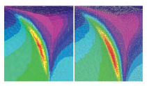 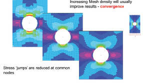 Figs. 9 (above) and 10 (right): Improving stress distribution and accuracy. |
Switching on stress averaging gives smooth contour plots, but the peak stresses are averaged. This is what I refer to in training courses as the "shell game." Where is the right answer hiding?
Accuracy Levels
An accurate estimate of stress levels in areas of concern is needed, such as around holes, fillets, weld toes and similar stress raisers. FEA loads and constraints may be applied to point or line features, instead of being spread over a surface.
In practice, any load or support is distributed over a region. Using a point or line implies a finite force applied on an infinitely small area, giving an infinite stress--a stress singularity. Unrealistically sharp fillets and welds also cause this.
Fig. 8 shows a fillet de-featured or undefined in the CAD model. The mesh follows the right angle corner. We can t manufacture that sharp a corner, theoretically down to molecular level. Our FE model is "dumb" in that sense--we defined an infinitely sharp corner, and mathematically, that s what we get. Increasing the mesh density to improve the distribution of stress and get a "better" answer won t work; the stress just keeps going up. This poorly modeled region can result in an arbitrary stress value.
If we include the fillet, as in Fig. 9 (left image), then we get a finite stress value. But the mesh may be too coarse. The mesh jumps are big, giving low confidence in the values. Increasing the mesh density results in only a small increase in stress and a good distribution (see Fig. 9, right). The solution is nearly converged. A study like this is very important to show accuracy of results.
Just Hit the Meshing Button?
We need to put the elements where they will be most effective--at stress concentrations with high stress values. We use manual controls, or an adaptive mesher, by running trial analyses and refining the mesh.
Fig. 9 (right) shows a local fine mesh at the fillet in a global coarse mesh, giving 208,826 elements. Using a global fine mesh gives 3,806,030 elements. The solution in CPU time is proportional to element number squared, so it is a significant increase.
The solution must fit into available memory. If we overflow, the FE solver writes to virtual memory or disc with a very sharp increase in solution time. This is known as the "cliff edge" effect.
| Achieving Perfection The perfect element shape is:
|
The amount of output data--stresses and displacements--can reach terabytes. Industry anticipates a rapid increase in FEA data output to petabytes, or 1,000 terabytes. A lot of that is unnecessary, however, and can be avoided by good planning.
Everyone has finite resources, so aim to work within those limits. You can explore your resource limits by building dummy "block" models meshed to death. Compare model size against run time and data storage, and tune your FE model size. For example, if 5.8 million elements trips you out of core memory with a huge increase in runtime, aim for around 5.2 million elements.
Slicing and Dicing
Fig. 1 shows a solid with additional slicing on faces, and through depth to improve the mesh distribution. The extra operations result in a CAD model that is not an efficient definition of the component--although it is a more useful, "FE-friendly" CAD model where we exert better mesh control.
Loading is applied on one quarter of the end lug, so a surface must be created to define this (see Fig. 1).
In summary, if you have a structure that is mesh-intensive, it is going to take some planning. Performance tuning exercises help by giving you a feel for how many elements your system can handle, and accuracy tests will help you understand what the element density and permissible distortions are.
Tony Abbey is a consultant analyst with his own company, FETraining. He also works as training manager for NAFEMS, responsible for developing and implementing training classes, including a wide range of e-learning classes. Send e-mail about this article to [email protected].
MORE INFO

Tony Abbey is a consultant analyst with his own company, FETraining. He also works as training manager for NAFEMS, responsible for developing and implementing training classes, including e-learning classes. Send e-mail about this article to [email protected].
Follow DEJoin over 90,000 engineering professionals who get fresh engineering news as soon as it is published.


About Us · Contact Us · Editorial Team · Advertising · Privacy Policy · Subscriber Services · © 2026 Digital Engineering 24/7 · Peerless Media