Simplifying FEA Models: Plane Stress and Plane Strain

Editor’s Note: Tony Abbey teaches live NAFEMS FEA classes in the U.S., Europe and Asia. He also teaches NAFEMS e-learning classes globally. Contact [email protected].for details.

A previous Desktop Engineering article (“Simplify FEA Simulation Models Using Planar Symmetry”) explained that even with powerful modern computers, there is often a motivation to use simplifying techniques in structural finite element analysis (FEA). This follow-up describes how two closely related methods can be used to take 2D slices through a complex structure at regions of interest. The resulting FEA models can give valuable insight into local stresses more rapidly and efficiently than a full 3D model. They won’t tell the whole story, but are valuable tools for the CAE engineer.

The two FEA methods are called plane stress and plane strain. Both use 2D planar elements that look like thin shell elements and are meshed using planar surface geometry.

Plane Stress Analysis

Fig. 1 shows the important facts about plane stress analysis. The structural region is assumed to lie in the 2D xy plane, with the third structural dimension relatively small. In the figure, this is the thickness in the z direction. Stresses exist in the 2D plane as sigma x, sigma y (direct stresses) and sigma xy (in-plane shear stress). Each of these stresses is constant through the thickness as shown in the inset. In addition there can be no stress in the z direction. This stress-strain material relationship is defined in 2D plane stress elements used in this type of analysis.

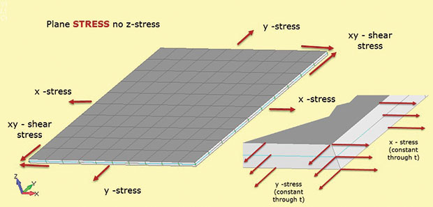Fig. 1: Plane stress; stress state assumptions.

The lack of z stress is the way to remember the element type designation plane stress (i.e. only in-plane stresses allowed). There are also no through thickness shear stresses. We could load the plane stress model in Fig. 1 with a bi-axial load and calculate sigma x and sigma y. There is no sigma z. We can also calculate the corresponding in-plane strains e-x and e-y. If we apply a shear load, we can find shear stress sigma xy and shear strain e-xy. Interestingly, we can also calculate the through thickness strain e-z. This is not zero, as the model is free to thin down in z as it stretches in x and y. There is no out-of-plane constraint to prevent this. In some solvers we can recover the through thickness strain e-z and use it to calculate the change in thickness. (If the model is in bi-axial compression then the z section will get thicker). This is usually considered a secondary strain and may not be available for output—but it is there and can be calculated manually if needed.

Fig. 2 shows an aluminum lug component. The lug protrudes from a composite sheet layup which has plies positioned and bonded over the tangs (or legs) and lower body section. The tangs transfer the load applied to the lug into the composite structure. In practice, the plies would be stepped to allow a smooth shear transfer through the bond into the composite. The shear transfer into the composite is simulated here by diffused surface traction forces “pulling” on the tangs. These balance the applied lug load.

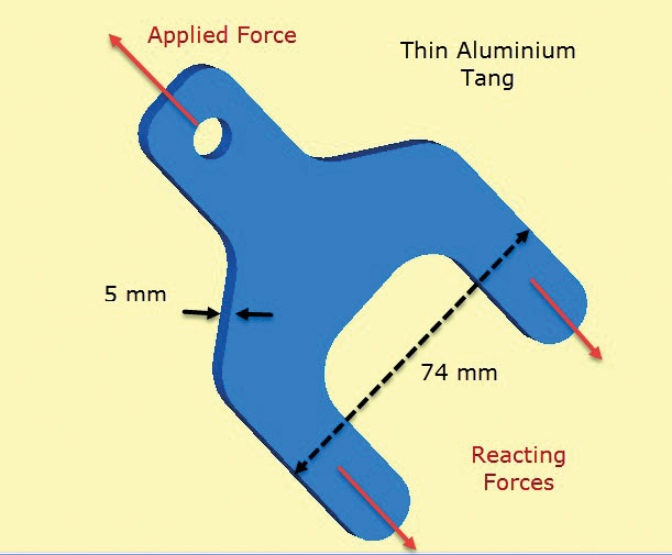Fig. 2: Thin-walled aluminum tang transferring load into composite structure.

The key assumption here is that through thickness stresses are zero and the in-plane stresses are constant through thickness in the component. This means the local detail of the shear load transfer from composite to tang is poorly modeled. However the focus of this analysis is to check sizing of lug and tang cross section clear of the composite, using in-plane stresses.

The thickness of the component is small compared to other dimensions. This value is input as the actual thickness in the plane stress element definition.

Fig. 3 shows the FEA model and the calculated maximum principal stresses. The areas of interest are around the lug and the shoulder radii. In the real world the stress state at the stress concentrations would be 3D and through thickness sigma z stresses and shear stresses would balance locally. However, it is very reasonable here to assume the in-plane stresses dominate. This is the same assumption implicit in most traditional stress concentration (Kt) calculations found in handbooks.

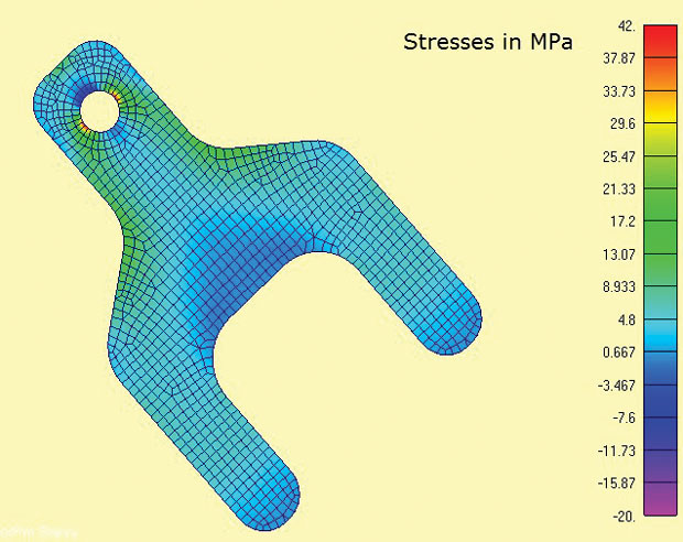Fig 3: 2D Plane stress elements showing maximum principal stresses

One of the convenient features of the plane stress analysis is that it is a strictly 2D analysis, so only three degrees of freedom (DOF) have to be constrained (in-plane translations x, y and rotation about z axis). This lends itself to the 3-2-1 minimum constraint method with balanced load. In a 2D case this degenerates to a 2-1 method. One node has DOF x and y constrained, a second appropriate orthogonal node has DOF x constrained. This allows the reaction load in the tangs to be applied directly as diffused balancing loads. It would be difficult to simulate this boundary condition via constraints to ground.

The through thickness e-z strain and hence thinning of the tangs could be calculated as a secondary effect.

Plane Strain Analysis

Fig. 4 shows the essence of the plane strain method. Again, 2D planar elements are used, but with subtly different assumptions. The in-plane stresses x, y and xy are developed as before. However this time it is the out-of-plane, or through thickness z strain which is set to zero. So plane strain analysis only allows strains in-plane. This works well to represent thick structures such as shown. The presence of this much material tends to stabilize the component and prevent it straining in z. This also means that constant through thickness z stresses are developed in the structure. This stress-strain material relationship is defined in 2D plane strain elements used in this type of analysis.

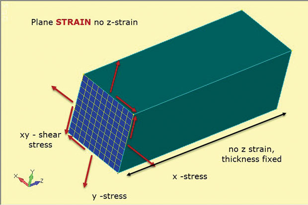Fig. 4: Plane strain analysis; stress and strain state assumptions.

The figure shows the orientation of the 2D plane strain elements as a cut section through a typical deep component. The assumption is that the stress state at this cut section will be duplicated at any xy plane cut (z station) through the component. The component is assumed to be prismatic (having a constant cross section) down its length.

In practice we use this method where the stress state is varying slowly from plane to plane in a deep component. There should be enough material through depth to stabilize and eliminate the through thickness strain. This is the same principle used on fracture toughness specimens shown in Fig. 5. A failure under plane strain conditions is shown for the center section of the thick specimen. The failure at the free edges and the thin section is a different mode, more like a plane stress state. A plane strain FEA model would by definition be a good representation of the centerline thick specimen behavior, but not of the free edges or the thin specimen.

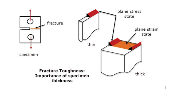Fig. 5: Fracture toughness specimens; thin and thick sections.

Fig. 6 shows another component used in a composite structure, forming a bonded joint. Here the section is constant and deep enough so that we can assume the stresses are also constant with depth. The free end surface faces (at +z, -z) will have a different local stress state (actually plane stress, as noted), however the objective of this analysis is to check the net section stresses on the centerline (z = 0).

The 2D plane strain analysis mesh is shown sectioned into the 3D component in Fig. 7. The section cut is defined at station z = 0.

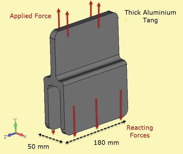Fig 6: Deep-section aluminum tang.

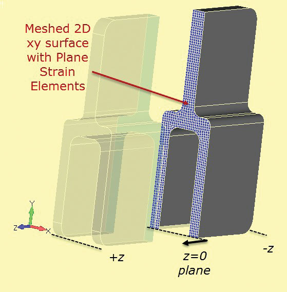Fig. 7: Section cut through solid section to develop 2D plane strain section.

A very fine 2D plane strain mesh can be used, which will run very quickly compared to a full 3D model. The 2-1 constraint method is used as before. The loading needs to be considered carefully. The “thickness” of the plane strain section is quite arbitrary, and is usually set at 1.0 by default. If the loading on the component is calculated as a running load through depth (N/m, Lbf/inch etc.) then this value can be used directly on the plane strain mesh. It is useful to pick a section, such as the single tang and estimate the nominal or average stress in this section for the full component. This can be used as a sanity check in the plane strain analysis. Incorrect loading is probably the main cause of error in this method.

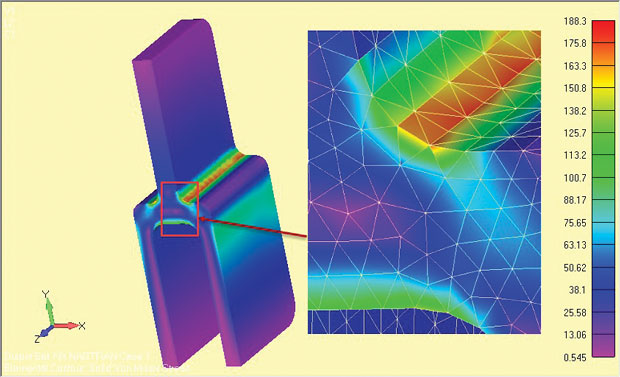
The results of the analysis are shown in Fig. 8 and show clearly the regions of high stress around the shoulder fillet. The stresses are valid for the central depth region of the component (z = 0).

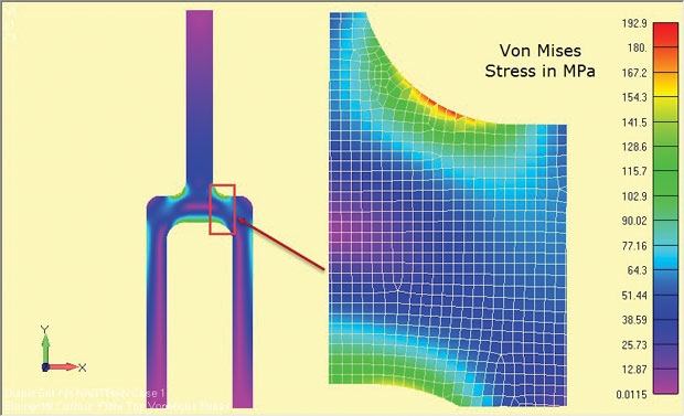Fig. 8: Plane strain analysis results of a deep tang component.

The stress quantities used will depend on the solver used. Some solvers ignore the z direction stresses as secondary and recover the in-plane stresses. The principal stresses and von Mises stresses then relate to a 2D in-plane stress state. If the z direction stress is recovered then it should be clearly identified, so that the 2D in-plane stress state in the x-y plane can be identified.

What exactly does the z direction stress represent? It is the stress developed due to the enforcement of zero z direction strain. The stress acts as if the free end faces of the prismatic section were fixed. At the central plane of a deep section component these will be the complementary stresses needed to hold the zero z direction strain state. In reality as we move toward the free surface faces, the z-stress drops to zero and becomes a plane stress distribution (as seen in the thick fracture mechanics specimen).

In many cases, such as a pressurized cylinder, the end faces are capped and will in fact develop an axial stress due to axial forces. This will be a different stress from the induced axial stress in the plane strain analysis. A hand calculation will be needed to calculate the axial stresses, or possible a supplementary axisymmetric model for pressure vessels.

The ease of geometry and mesh construction lends itself well to “what-if” studies or more formal shape optimization studies.

For comparison, a half symmetry full 3D analysis of the deep tang component was done and the results are shown in Fig. 9. The nominal stress across the upper single tang leg is identical in both cases—remember this is the basis of any sanity check.

Fig. 9: Full 3D model of the deep tang, showing stress results.

The local shoulder stresses are lower by a small percentage in the full model. This is for three reasons. First, the relatively coarse 3D tet mesh is inferior to the very fine 2D plane strain local mesh. A convergence check on the 3D model has not been carried out.

Secondly, there is a small change in geometry at the free surfaces (+z, -z) compared to the z = 0 section due to the end fillets. In this case, the effect is negligible as the fillets are away from the shoulder regions. In many components, however, there will be local fillets, and run out details. which will vary the geometry from a simple xy planar face. Local stress variations at free end faces may have to estimated or checked with a full 3D model.

Finally, the plane strain assumption of a fixed z constraint at +z,-z sections is not true for a finite depth component. The z stress will diffuse to zero at the “real” free faces. This effect is shown in Fig. 10, which uses the 3D model as is and also as a simulation of the plane strain z stress.

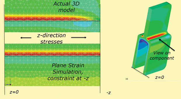Fig. 10: Diffusion of z-stress toward the free surface.

Fast and Efficient

Plane stress and plane strain analyses are useful 2D methods that can often supplement full-scale 3D models. Not all features can be represented, but with some ingenuity, stresses in key areas can at least be estimated. The motivation for using the methods is to enable fast efficient analysis with easy 2D geometry and mesh construction.