Helping design and engineering professionals discover, evaluate and specify technologies and processes that shorten the design cycle and enable success.
Alert!
Digital Engineering ceased publication on July 1, 2026. This website remains available as an archive of engineering content.
For inquiries or information, please email [email protected].

May 2026 Special Focus: Artificial Intelligence in Design and Simulation
In this Special Focus Issue, learn about the latest developments in the integration of artificial intelligence into engineering workflows.

Design & Simulation Software Guide 2025
In this Special Issue, Digital Engineering presents its second annual guide to design and simulation software vendors.
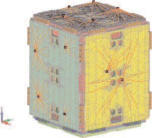 This is a satellite FEAmodel showing instrumentation attachment points (black squares) for idealized mass elements as defined by a center of gravity connected by rigid links (orange lines).Themodel is driven with an input power spectral density (PSD) function. |
If you’ve kept up with this series of articles, you now know more about the dynamic behavior of structures than 95 percent of your peer group within the design and engineering world. And after reading about how vibration analysis reveals key information about structural behavior (see DE, April and May 2008), the terms “natural frequencies, normal mode shapes, mass participation factors, and strain energy” have become integral to your vocabulary.
Up to this point the discussion has centered on qualitative terms about the mechanical response of structures due to dynamic loading. In this last part, we'll show how to extract real quantitative data (i.e., displacements and stresses) from a simple normal-modes analysis.
Doing It On the Cheap
The dynamic response of a structure is derived from its individual normal modes. If you hit your structure, its dynamic response is formed by the summation of its individual modes. Mathematically, we know that each one of our normal modes has a frequency, a mode shape, and a bit of mass associated with that shape (a mass participation factor). All of this data is derived from the basic equation of motion: ma+kx = 0
From this equation, the standard linear dynamics solution can be derived as:
v = K / m
where v is the frequency or eigenvalue of the system. Since no forces are involved in this equation we can't have any real displacements or stresses.
If we want real data, we need real forces as in: (ma+kx = F).
The brute-force approach is to solve the model in the time domain. A time-based displacement, force, or acceleration load is inserted into the model and then the computer makes a few thousand solves. At some later date, we then wade through piles of output data (remember, we are doing a complete solve at each time step) to figure out what went wrong, when, and where. This can be a daunting task and is often just plain impractical.
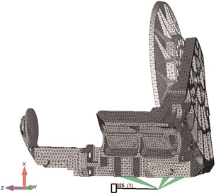 Figure 1: This is an image of an advanced optical platform for an airborne system placedon a virtual shaker table. |
If the loads are frequency-based (displacement, force, or acceleration as a function of frequency), then the door is wide open to all sorts of very numerically efficient solution strategies. First you perform a normal modes analysis and then apply a frequency-based load. A linear solve is made only at each normal mode or eigenvalue. The resulting displacements and stresses can be viewed individually or summed in some fashion to arrive at a combined damage response to the loading. The technique is extremely useful because you have reduced the number of solves from thousands to just a handful. Although we can't use this technique for every type of structure (linear behavior only), when you can use it, you have the ability to quickly gain insight into the dynamic behavior of the structure on the cheap (minutes versus days).
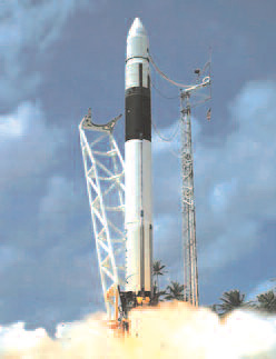 Figure 3a: A rocket launch and other chaotic events create vibration (acceleration) spectra that are best idealized in a statistical sensevia power spectral density functions. |
Modal Frequency Sweep (MFS)
Frequency-based loads are more common than you might think. Our previous example was of a vibratory conveyor. Since that was rather straightforward, let's look at something a bit more complex.
Figure 1 shows a high-precision optical-mirror assembly that will be attached to an airplane or helicopter. Airborne structures provide a vibration-rich environment with their high-speed gearboxes, jet turbines, rotating blades, etc. To assess the robustness of the design, you can perform a virtual shaker-table experiment. Our desired output is the deflection response at the focal point of the mirror under severe vibration.
Without having to build the mirror, you can input a sin sweep of 1g from 200 to 3000Hz to the model, and see what gets amplified or harmonically driven in the structure. Figures 2a and 2b show the output graph of acceleration and displacement as a function of frequency for the sin sweep.
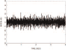 Figure 3b: The rocket acceleration measurementsare converted into a power spectraldensity function with units of accelerationsquared against frequency. The appliedload is based on frequency. |
The mirror system has eigenvalues at 710, 1292, 1570, 1996Hz, etc. But as shown in Figures 2a and 2b, only the mode at 710 Hz creates any real sympathetic accelerations and displacements. This is logical since this mode is aligned with the forcing function and has a mass participation factor of 35 percent in the direction of the forcing function. In a way, we knew what the results would be before we ran the analysis. But now we have real numbers.
Power Spectral Density (PSD) Analysis
Satellites are expensive and failure is even more expensive. During launch (Figure 3a) they get pounded by a broad and chaotic spectrum of vibrations (accelerations) from the rocket motor, stage separation, acoustical noise, etc. No single acceleration frequency dominates and there are multiple layers of noisy events that occur randomly.
To numerically model such loading, a statistical approach is used where acceleration measurements are converted into a power spectral density (PSD) function with units of acceleration squared against frequency (Figure 3b). Once again, we have a loading curve where the applied load is based on frequency.
|
The statistical nature of this calculation comes from the conversion of the acceleration time history data to the PSD function. The PSD amplitudes are actually root mean square (RMS) acceleration values that are fitted to a standard statistical distribution where the mean value is zero and what is plotted is the standard deviation versus frequency. As non-intuitive as this may sound, it is a very effective way to convert chaotic, random noise into a numerically useful load-function.
Analysis Checklist 1) If you review the normal mode response, its modes and its mass participation factors, you might not need these more advanced techniques. |
Another unique aspect of the PSD analysis is that all of the modes of the structure are assumed to be vibrating or excited by the PSD function simultaneously. Somewhat like a bell being rung, the output response is a summation of the amplitudes of all of the frequencies of the structure within the range of interest.
As an example, an FEA model of a satellite has various instrument payloads represented as mass elements. These payloads are attached to the main structure of the model with rigid links. In many cases, the utility of a PSD analysis is to determine the transfer function of the structure or how the satellite frame will transmit acceleration into the instrumentation packages.
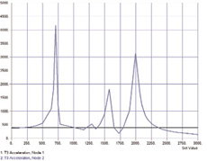
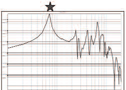 Figure 4: The output spectral density plot of the satellite analysis indicatesthe location of the first normal mode with the star marking 70Hz.The chart shows frequency on the x axis and PSD (g-2/Hz) on the y axis. |
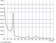
The resulting transfer function is just another PSD. We then use this output to perform a more detailed PSD analysis on the instrumentation package to determine whether it will survive launch.
The dominant mode of the satellite is around 70Hz (Figure 4) and the output PSD function reflects this fact with a huge spike at this frequency (marked with a star). If we knew that our instrumentation package was susceptible to frequencies at 70Hz, our design solution would be to develop a stiffer satellite frame that would not have a dominant normal mode at 70Hz. Even without the PSD analysis, a clear understanding of the normal mode frequencies, their mode shapes, and corresponding mass-participation factors allows you to make valid predictions.
Now you have the concepts, the vocabulary, and the big picture for operating in the world of linear dynamics. A simple modal analysis can put you well on the way to successfully meeting your structural engineering challenges. Why not give it a try?
George Laird, Ph.D., P.E. is a mechanical engineer with PredictiveEngineering.com and can be reached at [email protected]. You can send comments about this article to [email protected].

DE's editors contribute news and new product announcements to Digital Engineering. Press releases may be sent to them via [email protected].
Follow DE


About Us · Contact Us · Editorial Team · Advertising · Privacy Policy · Subscriber Services · © 2026 Digital Engineering 24/7 · Peerless Media