Dynamic Analysis

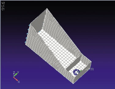Fig. 1: Tray support structure.

After 35 years, I still find dynamic analysis to be a “buzz,” if you will excuse the pun. There are so many uncertainties in dynamic analysis, dependent on the way that the mass distribution, the stiffness distribution, loading forms and constraint forms all interact. The results of an analysis are often a surprise, and always need checking.

Natural Frequencies and Mode Shapes

The natural frequencies of any structure are special frequency values where the interchange between kinetic energy and stored energy occurs most readily. A simple suspended mass on a spring has a single natural frequency, say 134 Hertz (Hz). Hertz units are in cycles per second.

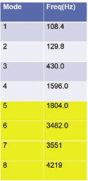Fig. 2: The first eight natural frequencies of the tray.

The stored energy is a maximum in the spring when pulled away from the datum position before release. After release, the kinetic energy builds up as speed increases. It is at maximum when the mass is traveling fastest as it passes through the datum position. At this snapshot in time, there is no stretch in the spring, so stored energy is zero.

Beyond the datum, the spring stiffness opposes motion—and the stored energy builds up, speed drops and kinetic energy falls. The spring comes to rest at full stretch, with maximum stored energy. That is half a cycle of motion completed. The whole process is repeated indefinitely if no damping is present.

The readiness of the structure to “flip-flop” between energy modes is what makes the natural frequencies so important. It means the structure will respond to an external excitation most aggressively at these values.

For a more complex spring mass system, with three springs and three masses suspended, the model now has three degrees of freedom (DOF). We will find three possible natural frequencies of increasing value. For a large model with 100,000 DOF, theoretically there are 100,000 natural frequencies. Luckily, most structures only have significant response at the lowest modes.

Associated with each natural frequency is a mode shape. Imagine the mode shape as a frame from a high-speed video or the “frozen” image seen by a strobe light, set just at the natural frequency. This is a deflected shape that is unique to that particular frequency. This uniqueness, or “orthogonality,” is also a very special property and we use it a lot in dynamics.

The structure shown in Fig. 1 is a simple cantilevered tray. It supports a piece of equipment modeled as a lumped mass connected to the base of the tray with a rigid, spider-type element.

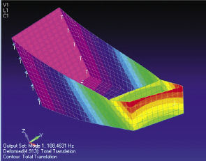Fig. 3: Tray mode 1, torsion at 108.5 Hz.

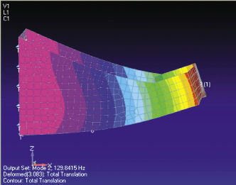Fig. 4: Tray mode 2, vertical bend at 129.8 Hz.

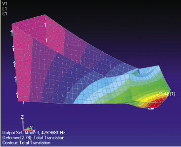Fig. 5: Tray mode 3, local base dishing at 429.9 Hz.

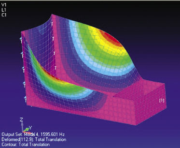Fig. 6: Tray mode 4, side walls bending out of phase at 1,595.6 Hz.

The first eight natural frequencies of the tray are shown in Fig. 2. There are approximately 5,000 DOF in this model, but mode 5,000 is of no interest to us as it is some random perturbation of the structure, rather like Brownian motion.

Associated with each frequency is its mode shape, and the first four for the tray are shown in Figs. 3 through 6. It is important to identify what the mode shapes represent and to describe them clearly. If we just refer to “Mode 2, 129.8 Hz,” we have no way of comparing it to test or other analyses. Its physical meaning gets lost in any report. The modes are described in the figures. You can make up your own terminology, as long as it is consistent and gets across the physical shape.

The higher-frequency modes are shown in Fig. 7.

What modes are important? That usually depends on the frequency range of the excitation forces. If the tray is connected to a solid bulkhead that is being vibrated up to 850 Hz, all modes up to that value should be included. However, mode shapes tend to interact—and we may find that the natural frequencies above the 850 Hz cut-off play a role as well.

Notice Mode 4 at 1,596 Hz (Fig. 4). We don’t hit this mode at resonance in our excitation range, but there may be some influence at 850 Hz. We really don’t know until we do a full response investigation, so a safety factor of one-and-a-half to two times the highest frequency is used. If we use a safety factor of two on 850 Hz, then Mode 4 at 1,596 Hz would be considered.

If the excitation is a force-impacting, rather than a steady driving frequency, it becomes more difficult to assess important modes. For example, a sharp triangular load shape through time has a lot of high-frequency content (remember the Fourier series from college days?).

However, a modal survey such as we have carried out provides great physical insight into the potential nature of any dynamic response of the tray.

Building Blocks

It is vital to carry out a modal survey as shown on any structural model before we carry out a dynamic analysis involving some type of external excitation. Whether we shake it or hit it, a structure will respond by combining the mode shapes together through time, or across frequency.

In our tray, we can see major modes associated with whole structure motion at 1 and 2; local dishing of the payload region at 3 and a local wall mode at 4. Higher-order wall modes occur at Modes 5 and 6, and whole-structure torsional modes occur at 7 and 8. This should give us a good, intuitive feel for response to any type of input.

Internally, in the solution of dynamic response finite element analysis (FEA), there are two approaches possible:

1. Modal method reuses the data from the mode shapes in a previous normal modes analysis step.

2. Direct method calculates the responses using overall system matrices, without needing a normal modes step.

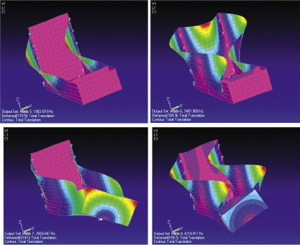Fig. 7: Modes 5 - 8, above frequency range of interest.

When using a direct method, there is a temptation to ignore the need to do a modal survey because the calculation process doesn’t need it. This is a very dangerous practice, because without a modal survey you are “shooting blind” in any response analysis, with no way of knowing whether the model is showing the correct modal behavior. So please treat this as a two-step analysis: Run a normal modes analysis to carry out a modal survey, then do a direct response analysis as required.

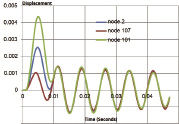Fig. 8: Time history of payload and corners in z.

We will discuss the pros and cons of modal and direct methods in a future article. The key thing to remember for now is that both are tools in the toolbox, and you can use both to build confidence in the results.

Time-based Response

Once we have understood the inherent modal characteristics of a structure, we can carry out a time-based (transient) analysis. The loading is applied through time, and we calculate the response through time. Fig. 8 shows the vertical response through time of the payload mass and two corners of the tray. A rectangular pulse was applied for 0.01 seconds at the payload. The orientation of the load was at 45 ° to the vertical.

The response during loading is shown; notice the spread of values as a torsional response is seen initially. When the load is removed, we see a steady wave form. It has a dominant frequency and is slowly decaying. We can measure the peak-to-peak values to give a time period.

The inverse is the frequency, so we can check against the natural frequencies of the structure. We are looking for confirmation of the frequency and corresponding mode shape. If it all ties up, we build confidence in the model.

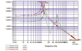Fig. 9: Frequency response of the tray at payload position.

The decay rate is proportional to the damping we model in the system. Damping is a complicated subject, and we will explore it in more detail in a future article. However, most damping is modeled using a viscous (velocity-dependent) simulation. By using successive peaks, we can check the damping level defined.

It is best to check a large model by using xy plots at key positions as shown. Only then do we perhaps need to do a full animation of the model. A full animation takes up a large amount of data storage, and a very large model can defeat a post processor’s capabilities. These may be “nice to have”—but xy plots and frozen time plots can usually tell a full story.

Frequency-based Response

An alternative to a time-based solution is a frequency-based solution. A typical application would be a structure connected to a bulkhead or similar base structure, which is being shaken across a frequency range. This does not represent one physical event, but represents an exploration of the structural behavior across a range of possible steady-state responses.

A shaker table is a good analogy: We mount the structure on the table and vibrate at 10 Hz. We ignore the start-up motion, and concentrate instead on the peak displacement, acceleration, stresses, etc., at the steady-state response. We then increase the frequency to, say, 20 Hz—and wait until the system settles down and measure the peak steady-state responses.

Alternatively, we can imagine a point load introduced to the tip of a beam via a “stinger.” The stinger oscillates at a set frequency, and when the system settles to steady state, we measure the peak beam response. We change the frequency and repeat the process. Similar external excitations can be set up on more-complex structures.

Fig. 9 shows the displacement response of the payload point on the tray when the payload is driven at a range of input frequencies. The response in x, y and z is shown. From this, we can see the influence of each of the modes we investigated earlier, and we would check that the payload directional response ties up with the survey.

We can plot a similar figure for acceleration response, and we can use these in the design assessment. For example, if the driving input at the payload is 200 Hz, this means the response is low—nicely between peaks. The y (lateral) direction response is dominant at 108.5 Hz Mode 1 torsional response. The z (vertical) response is less severe, at 129.8 Hz vertical bending Mode 2. This information could be used to check fragility of the payload.

This has been a very short introduction of a very broad subject. The main emphasis is on the importance of the calculation of natural frequencies and modes’ shapes of a structure. These are inherent characteristics of any real structure. Any time- or frequency-based response analysis is dependent on how accurately these are represented. To aid our understanding and build confidence in any dynamic analysis, a full modal survey should be carried out.

A time-based transient solution is the most intuitive type of dynamic loading, and represents a specific loading case. A frequency-based solution, on the other hand, is usually a search across a potential applied loading range for the most damaging steady-state loading. DE

Tony Abbey is a consultant analyst with his own company, FETraining. He also works as training manager for NAFEMS, responsible for developing and implementing training classes, including a wide range of e-learning classes. Send e-mail about this article to [email protected].

More Information

FETraining

NAFEMS