Solving for Defective Units

By David Lengacher

 

Engineers make decisions and solve problems every day, but sometimesthe optimal decision or solution is counterintuitive. Consequently,this class of decisions can very often have considerable financialimpact on a company. For almost every problem encountered in industrythere is a corresponding methodology or algorithm for pursuing theoptimal solution. The challenge engineers face is trying to match theproblem with the correct methodology. This article will explore onesuch problem that is shared by several seemingly unrelated industries:how to identify defective product before it’s shipped to the customer.

It is easy to imagine that many engineers and data analysts,particularly those involved in the manufacturing and chemical processindustries, have found themselves addressed by a supervisor in thefollowing manner:

“Hey, ]say your name], for the last three months we’ve seen a spike indefective units returned by our customer. A hundred percent of theunits we’ve produced and shipped in the last three months are withinthe customer’s design specs, but a number of the units fail withinhours of the customer using them.

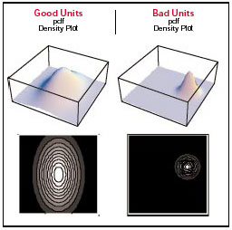
“We measure and record two environmental conditions that each unit isexposed to during the production process. Here is what we foundregarding the distributions of the returned defective units versus goodunits.”

This is where he pulls exhibit A (see table below, right) out of thin air andshows itto you.
“Now, I’m not a statistics expert,” the boss continues, “but I thinkit’s obvious that the defective units are not ‘different enough’ for usto separate them from the good units because it appears thedistributions will overlap.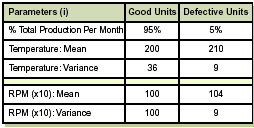

“Since inspection won’t do any good because no units are produced outof spec, what we need is a formula that will internally fail high-riskunits, based on production environmental conditions, so they don’t getshipped to the customer. The goal here is to minimizemisclassification. Right now we’re classifying 100 percent ofproduction as good, but we know 5 percent ends up being defective, sowe’re misclassifying 5 percent of everything we produce! Do you thinkyou can come up with a formula that will minimize misclassification andbe prepared to defend your methodology, by lunch?”

Gulp. “Uh, O.K.,” you answer, almost quivering. “I’ll see what I can do.”
You know that the problem you need to solve is to take an x, y plane,the production environment plane, and divide it into two regions: 1)Pass and 2) Fail. To get an initial visualization, you grab somemarkers and a ruler and draw what you think the distribution looks likeon your dry erase board to see if they overlap. You try to plot themeans, two standard deviations, and where you think the decisionboundary that minimizes misclassification would be.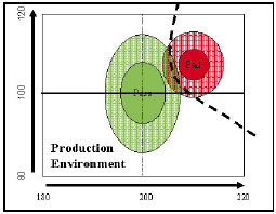
Logically, you think you should try to divide the overlap between thetwo classes and draw your decision boundary so that it splits theoverlapping region. Next, you consider everything above the line asyour failure region. This seems easily defendable and you think yourboss will be impressed with such a quick solution. But then youremember the Statistical Pattern Classification class you took incollege and remember something about Bayesian Decision Theory.

After some quick research on Bayesian theory in your old collegetextbook, you find the solution to your problem. In order to minimizemisclassification between two distributions you need to find theprobability density functions of each distribution, find the log ofeach, add to each the log of the corresponding prior probabilities, setboth equations equal to each other and solve. This will produce thedecision line that will minimize misclassification.

There’s no example of this in the textbook, but after some digging inother statistics books you find the following equation (see below),referred to as a discriminate function, that is the equivalent to thelogarithm of the probability density function of any multivariateGaussian distribution with the log of the prior probability alreadyadded on. This does not seem as complicated as the description in thetextbook because there are only two variables that need to be enteredand you already recognize what they are: S is your covariance matrixand m1 is just your mean vector. And your boss gave you both of those,so this is going to be easy. You read that D is just the dimension ofyour Gaussians, so this will be equal to 2.

Some notation is unfamiliar because it’s been a while since you’vetaken linear algebra, but after asking a fellow engineer in theadjacent cubicle, she reminds you that:

1)S-1 is the inverse of your covariance matrix
2)Det]S1] is the determinant of the covariance matrix

Next, you simply plug in the corresponding S and m1 components and produce yourtwo equations (below).

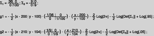
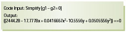
You know that since you have both Matlab and Mathematica on yourdesktop, you don’t need to compute any of these components yourself.Now you just set the equations equal to each other and solve for x andy to get the equation that is your optimal decision line.

Before you plot this line you remember that you have yet to see whatthe true distributions look like in 3-D. So far you have only sketchedthem on your dry erase. Using your software savvy, you produce thefollowing graphs using Mathematica:

Now you can plot your decision boundary and you quickly realize theboundary is nothing like what you had predicted. It’s much smaller andfully encapsulated by the Passing Region.

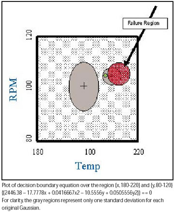
Surprisingly, the red region shown here tells us that we should onlyfail units that fall in this region. For example, if you were asked toclassify a unit represented by the green dot, then you should not failit even though it is very near the center of the distribution of thefailed units. This is very counter-intuitive. This is due to twoimportant numbers: the prior probabilities of 95 percent and 5 percent.Let’s see what the failed region would look like if both good units andfailed units are occurring in equal quantities, thus having equal priorprobabilities.

Hypothetical Case:

Defective units and good units are equally likely to occur (prior probabilitiesof 50/50).

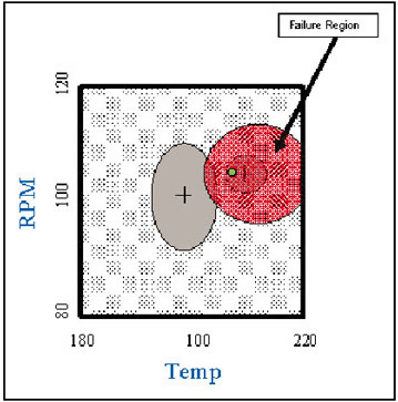
Now this looks similar to your original idea. But because defectiveunits only comprise 5 percent of the total production, you have to takethis into account when classifying your products internally.

Now you have a statistically sound model to present to your boss and you’ve doneit all within an hour!

David Lengacher is currently working in modeling and simulation inWest Lafayette, Indiana. He has an MBA from Purdue Universityand an MSin Operations Research from the University of Florida. To contact himabout this article, send an e-mail [email protected].