Symbolic Computing for Design Engineers

By Dimitrios Karamanlidis

Author’s Note: While we used a particular computer algebra system, namely Maple, every computation performed could have been done using any other system.

For someone to claim that “engineering” and “computing” are synonymous would certainly be an incorrect statement. After all, there’s much more to engineering than just computing. Replace, however, “synonymous” with “like twins”  “and everyone around you is nodding in agreement.

Now, more often than not, when engineers refer to computing,  they mean “number crunching” of some sort or another. And nowadays, the ubiquitous tool to do that is most likely MATLAB (and to a lesser extent,  perhaps, MathCAD). No reasonable person should have a problem with that. Engineering is, after all, a problem-solving profession “and at the end of the day, you need concrete numbers to build something. But there is another angle to it, and the purpose of this article is to showcase, on the basis of some examples, that there are a good many situations during an engineer’s workday in which using symbolic computations is the smarter choice. Let me explain.

What’s Symbolic Computing?

Let’s venture down memory lane and recall that in high school we were introduced into algebraic equations, something like: 3 * x - 15 or,  more generally a * x = b In both cases, we were able to solve for the unknown, x, and get, respectively: X = 3 and x = b / a. Little did we know back then that in the first case, we performed numerical computing (“number crunching”), and in the second case symbolic computing.Once we mastered that subject, we were taught how to solve simultaneous algebraic equations, that is, math contraptions of the form: A x = b where A represents the coefficient matrix, b the vector of known terms, and x the vector of unknowns. Both A and b could contain numbers and/or symbols. Either way, when the solving was done longhand, it always meant lots of tedious, time-consuming work “so much so that anything with more than, say,  three unknowns was not to be attempted by mere mortals. The advent of electronic calculators and later, personal computers shook things up “in that technology made it possible for everyone to solve for many unknowns without much effort. That is, as long as A and b contained numbers and numbers only. It was that limitation that led to the creation of so-called Computer Algebra Systems (CAS): software able to handle symbolic computing in conjunction with things such as algebraic systems of equations, differential equations, integrals and differentials and so forth.Excellent, you say, but why is that such a big deal for someone who is not a math major, but an engineer?Bear with me! Suppose you’re working on analyzing/designing some truss structure and wish to evaluate the performance of several variants in terms of cross-sectional and material properties, loading conditions, and the like. Tackling the problem by way of numerical computations (say, standard finite element analysis, or FEA) would prove quite wasteful, for it would require a slew of computer runs to go through the various “what-if” scenarios.Now enter symbolic computing. In that case, you treat the various design parameters (lengths, angles, areas, load magnitudes, etc.) as variables, and proceed to obtain explicit formulae for all output (displacements, stresses, internal forces, you name it).What is the advantage? First, having these formulae in front of us makes it possible to grasp more easily which parameter(s) influences the response the most. If, due to the complexity of the problem, mere inspection is not an option, we could resort to graphical tools. Second, it requires little effort to plug into the derived formulae any amount of numerical values and obtain the respective results without the need to reanalyze.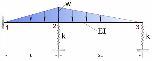  

Figure 1: Spring-supported cantilever.

On with the Show

With the “tell” part taken care of, let’s now deal with the “show” part “and turn our attention to a couple examples. First, let’s look at some mechanical part/system which, in idealized form, may be represented by the model depicted in Figure 1.There are a number of possible scenarios that come to mind regarding this problem, including:

• How are bending stresses and deflections affected by certain variations regarding geometry, stiffness and loading?
• For a given configuration, in terms of geometry and stiffness, what is the maximum load magnitude w allowed if certain design criteria pertaining to maximum deflections and/or stresses are to be met?
• For a chosen configuration, in terms of loading and geometry, what is the lightest (“most economical”) beam section one could select “provided that certain upper limits for stress and deflection will not be exceeded?
 

How do we go about solving this problem symbolically?  Perhaps the most straightforward approach is to set up an FEA model whereby stiffness matrices and load vectors are expressed in terms of the variables depicted in the figure, namely w, k, EI and L. For simplicity, we choose just two standard beam elements to represent the structure, which results in a total of four degrees of freedom (DOF). In other words, we get a deflection and a rotation at each of the nodes 2 and 3.

Following standard procedure, we then arrive at the augmented stiffness matrix, A, and load vector, b, shown below: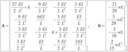

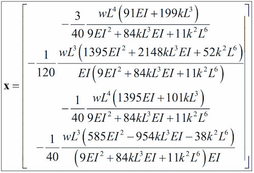
Based on that, the obtained symbolic solution reads as:

From this, all relevant system response data such as internal forces/moments, stresses, support reactions, etc., may be computed. Because we have derived explicit formulae, we could plug into them any number of numerical values. Here as a simple demo, we choose to vary the spring stiffness k and observe the effect it has on location and magnitude of maximum stress. It turns out that for large values of k, the maximum stress becomes several times smaller than the value obtained for k=small. Also,  its location shifts from the fixed support to the first spring. The graphics in Figure 2 depict, respectively, the shear force and bending moment diagrams for k=large.

 

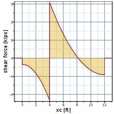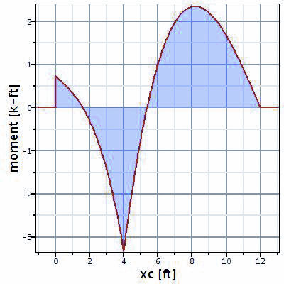Figure 2: Shear and bending moment diagrams.

Now, as a second example, consider the dynamic system depicted in Figure 3.

 

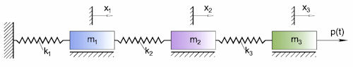Figure 3: Dynamic system with three degrees of freedom.

Typically, in a situation like this, one is interested in the following:

a. eigenfrequencies and eigenvectors, which control the free vibrations of the system; andb. steady-state response from externally applied loads.To accomplish the above, we must formulate the equations of motion of the system. One approach that works particularly well in conjunction with symbolic computing is the method of Lagrangian equations (typically covered in a basic, sophomore-level college course on “Dynamics”). This results in three ordinary differential equations, in terms of the three unknown deflections, which in compact (matrix) form read as: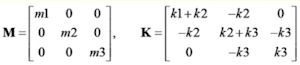 where and

As far as notation goes, M and K are,  respectively, the mass and stiffness matrix of the system, and p denotes the load vector. Further, an overdot denotes differentiation with respect to time, so a double overdot on x denotes the acceleration vector. To keep the formulae resulting from the symbolic analysis manageable, the following (arbitrary) choices were made for the system parameters:

m1 = m, m2 = m, m3=m and k1 = 2*k, k2 = 3 * k, k3 = k with which the eigenfrequencies of the system were found to be: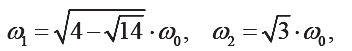

The respective normalized eigenvectors are depicted in Figure 4, whereby the masses are represented by a solid circle. The distance of each mass from the y-axis (abscissa) represents the normalized amplitude of vibration for that mass.

 

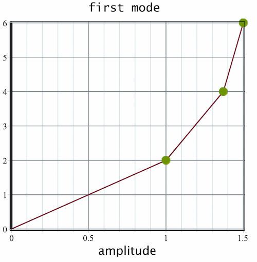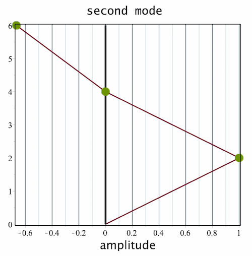Figure 4: Normalized eigenvectors.

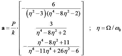
  Typically, free vibrations die out quite quickly because of the presence of some damping (either external or internal) in the system. For design purposes, what is usually more important is the system’s steady-state response to externally applied loads. Here, we choose the excitation to be in form of a harmonic load (frequency W, amplitude P), acting on the third mass only. By solving symbolically the (matrix) equation of motion, the amplitude vector for the three masses is then found to be

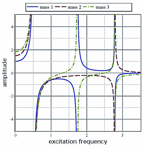
As is customary, the three amplitudes are plotted versus the excitation frequency, leading to the diagram shown in Figure 5. In this diagram, the following features are worth noting:

 

Figure 5: Amplitude-frequency diagram.

• When the excitation frequency matches one of the system’s eigenfrequencies, resonance, that is very large amplitudes occur.
• When the excitation frequency reaches a value equal to the second eigenfrequency, resonance occurs only for masses 1 and 3,  whereas for mass 2 the respective amplitude is rather small (“vibration isolation”).
• The amplitude curve for mass 3 intersects the zero-axis at two locations, meaning that for these two frequencies, mass 3 does not vibrate at all.
 

In summary, we have shown on the basis of two examples how symbolic computing may be used to perform engineering-related calculations. The advantage of symbolic computing vs. number crunching lies in the fact that the obtained results are in form of general formulae, and thus do not depend on specific numerical values.

Dimitrios Karamanlidis, Ph.D., received his education in Germany. His professional career spans more than 30 years as a researcher, teacher and consultant in the general area of CAE. He’s currently a faculty member in the College of Engineering at the University of Rhode Island. He may be contacted via [email protected].

More Info

Axiom Maple MathCAD Prime Mathematica Mathomatic MathWorks Maxima Reduce