FEA Case Studies: Check Models and Identify Errors

Editor’s Note: Tony Abbey teaches live NAFEMS FEA classes in the US, Europe and Asia. He also teaches NAFEMS e-learning classes globally. Contact [email protected] for details.

This month’s article is a follow-up to the two-part DE series on Accuracy and Checking in FEA (finite element analysis) models (January 2014 and February 2014). Several case studies are shown where errors have crept into the modeling. We look at how to identify the errors, as part of our normal checking routine, and subsequently how to debug and correct the issues.

Many modeling errors are simple data entry mistakes, others are more complex and involve constraint boundary conditions, meshing problems or misunderstanding of the physics involved in the simulation. The range of potential errors is vast—ask any FEA support engineer! We are investigating a small subset here.

Case Study 1: Loaded Crank

The crank model and loading setup shown in Fig. 1 was used in the February 2015 article on Free-Floating models.

Fig. 1: Configuration and loading for case study 1.

The FEA model uses the 3-2-1 method to put the structure into minimum constraint to support a balanced set of loads. In the new case study, the analysis is run and the stresses and deflections checked as shown in Fig. 2.

Fig. 2: Stress and Displacement results for case study 1.

The stresses look all right, and agree with the distribution and peak magnitude (69,437 psi, 478.8 MPa) from the previous article. It is tempting to leave it there and carry on with writing the analysis report. However, two items must always be checked first with any FEA result: stresses and deflections. The distribution of deflection is shown in the deformed plot, and can be animated for more clarity. In our case the deflection is relative to the fixed horizontal clamp face. The loading action of the actuator rod causes the vertical arm to translate and rotate. Because the constraint system is not relative to the crank pivot, the crank pivot appears to move relative to the clamp face. This is acceptable in the model and is expected behavior, but it is worth thinking about carefully. You may have to explain to a client or manager why the crank is not showing “realistic” motion.

Many post processors have the ability to plot all displacements relative to a target nodal displacement. This is very useful in understanding the deformed shape, particularly in cases such as ours. We do however need a node at the center of the pivot, which is coupled into the analysis, but does not change the stiffness or load path of the model. It just acts as a datum. We can use a “flexible spider” type element for this purpose (sometimes called a load application element). This is shown in Fig. 3. We can create a center node and connect it to the inner faces of the pivot with the spider. The spider adds no stiffness. The node will displace as a type of least squares average of the motion of the pivot face nodes. It acts as a tracking node and is just what we want as a relative position. The displaced shape plot in Fig. 3 is now set as relative to the new pivot center node. The post processor calculates all deformations relative to this point and the plot is much more understandable. Flexible spiders are excellent tools for this and similar type of situations where a datum or reporting point is needed.

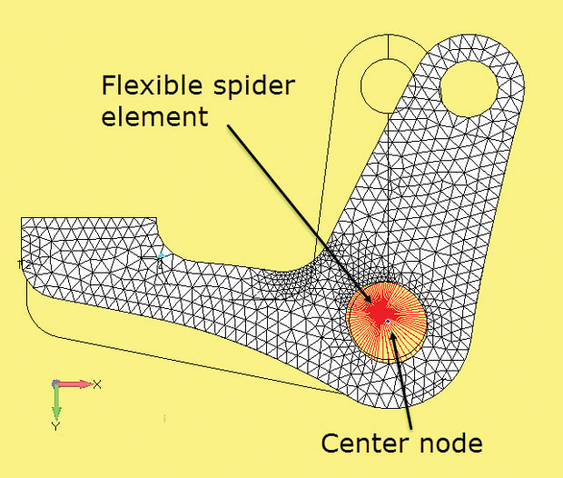Fig. 3: Spider element added with center node to give a meaningful displaced shape.

So far we have focused on the sense of the deformation. However the scale of the deformation is equally as important. In Fig. 2, the peak deflection magnitude is reported in the legend on the screen shot. The value may be shown in a summary file, or require a result probe of some kind. The displacement in our case is in inches—and is therefore a very suspicious value of 9.649 in. (245 mm). This is obviously an error as it is so large, but in general we should have in mind what would be a typical ballpark value for our structure. A stiff structure like this is going to have deflections in the order of thousands of an inch (0.003 mm).

We have identified the problem, what might have caused it? A quick checklist includes:

• Wrong material properties

• Wrong loading

• Constraint error

• Boundary condition stiffness error

We start first with the simplest to check: material properties and loading. The loading seems OK initially as the stresses are acceptable. A quick look at the material properties shows an error with Young’s Modulus set as 2.9E4 psi, not 2.9E7 psi for AISI 4340 Steel. For a simple rod the relationship between deflection d and applied force P is given by P=(AE/L)d, where A is the cross sectional area, E is Young’s modulus and L is length. So a factor of 1E3 down in E results in a factor 1E3 up in d. The correct peak deflection value is .0096 in. (.245 mm).

The stress relationship to applied force is just stress = P/A. So stress is insensitive to errors in material property in our simple case. In fact in more complex structures with parallel load paths having different materials (multiple E values), the relative stiffness will change with an error in one E value. The stresses may then be in error as too much load is attracted to the higher E value material.

If we wanted to check further we could pull out the reaction forces and make sure the value balances the load we think we have applied. However, for the 3-2-1 method that is not meaningful as the applied loads balance to zero by definition. We could overcome this by setting up two dummy models. The first constrains the pivot point face nodes only and applies clamp and actuator loads. The second constrains the clamp and actuator connection regions and applies load through the pivot. This splits the loads and allows separate checking of each. The loading and load paths for the 3-2-1 model are therefore effectively checked. Other complex load paths can be checked in a similar manner.

Case study 2: Yoke with Seeker Head

Fig. 4 shows a Yoke with Seeker Head FEA model. This has been explored in the two DE articles on Dynamic Response (May 2015 and June 2015). The Yoke is fixed to ground at its base and the Seeker Head is modeled as a lumped mass connected to the inside bearing faces of the pivot points.

Fig. 4: Yoke and Seeker Head model showing lumped mass idealization.

In our case study, a static inertia load is applied to the structure. The resulting stresses and deformations are shown in Fig. 5.

Fig. 5: Yoke and Seeker Head stress and deformation result.

From Fig. 5, the deformation looks very high at 0.625 in. (15.9 mm). A stiff cantilever structure like this would be expected to have less deformation. The stresses also look high. This seems like a sweeping statement, but we can relate the stress level back to the yield stress of the material. Yield stress is 215,000 psi (1482 MPa), we have three to four times that value. In this situation several questions arise:

• Has the material yielded in practice, if so we need a nonlinear material analysis to understand the level and extent of plasticity?

• Is the structural design anticipated to be significantly under strength?

• Are the loads applied correctly?

The significance of the first point is that a stress much more than 1.5 to two times yield is physically impossible and can only occur with significant plasticity. In that case a nonlinear analysis is the only valid solution. A linear analysis will be completely wrong.

The second point indicates an engineering judgment. Can the design be that bad? How have previous designs worked? Can a ballpark hand calculation show an acceptable design?

If the answer to the second point is that the structure is anticipated to have reasonable strength, then suspicion falls on the third point. The loads are very likely to be overly severe by mistake. The fact that the displacements are way too high tends to confirm this.

In this case there is a slight twist in that inertia loading is used. The relevant loading factors are 15g in x, 30g in y and 10g in z. Inertia load is developed throughout the body by multiplying each element mass by the body acceleration. So the mass or the acceleration may be in error. Using the principle of checking the simplest item first, we inspect the following data:

• Material density

• Reported volume and mass of the Yoke mesh

• Lumped mass of the Seeker Head

The material density is easily checked and is correct at 7.33145E-4 lb. mass/in3. The volume of the Yoke mesh is 16.6 in3 and gives a correct system mass of 0.0124 lb. mass. The lumped mass Seeker Head representation is 60 lb. weight, 0.15528 lb. mass. One point here is that the mass moment of inertia of the Seeker Head has been ignored. This may be a consideration when the debugging is completed and should be corrected. It is a secondary effect at the moment.

So it all points to the loading input! There are two approaches now; checking the raw input data as well as the reaction forces. Checking the raw input is easiest so is carried out first. A check reveals that the load levels have been factored by 10 in error and are 150:300:100 not 15:30:10. This kind of error when manipulating and preparing load data is quite common – I have done it many times!

A straight linear scaling by 0.1 gets us down to 0.0625 in. (1.59 mm). The loading is severe and therefore this order of deflection seems reasonable for a cantilevered beam. We can check by running a 1g in x direction case and comparing with a simple hand calculation. The deflected shape plot in Fig. 5 also shows evidence of twisting as well as bending under the combined loading, which is a useful sanity check.

The stresses now scale down to peak Von Mises of 72,951 psi. It is a high stress, but the loading is severe. A hand calculation could easily check the values here at the base of the Yoke. Knowledge of similar successful designs would reinforce that the design was feasible and hence the FEA result is sensible.

Case Study 3: Tang Half Symmetry Model

The Tang model shown in Fig. 6 is a variation of the model used as a 3D verification in July’s DE article on plane stress and plane strain. It features a half symmetric model that is loaded on its top face and constrained on the two lower faces, so that a load path through the fork section is created. In this case the geometry is created from three separate bodies. The geometry is meshed and a linear static analysis is created. Automatic linear glued contact is created between all mating surfaces (body 1 to body 2 and body 1 to body 3).

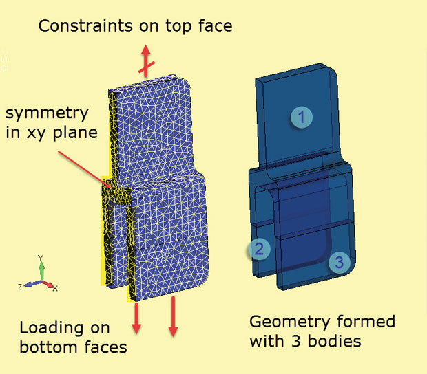Fig. 6: Geometry and mesh of Tang model.

The resulting analysis ends with a failure message reporting an excessive pivot ratio. An excessive pivot ratio discovered during the matrix solution process indicates that the highest and smallest Degree of Freedom (DOF) stiffness terms are too widely separated. The system default is exceeded and the analysis is stopped automatically. If the analysis were to continue it could reach a point where the solution “blows up” with a near divide by zero operation. The results from such an analysis would be unusable.

Our task is to find the cause of the excessive pivot ratio. The likely reasons include:

• The model is not fully constrained in all DOF—resulting in rigid body motion.

• Cracks are occurring in the mesh—resulting in rigid body motion.

• Material properties are incorrect—giving high and low stiffness terms.

• Elements are highly distorted giving spurious high and low element stiffness terms.

• DOF are cross-coupled in error by multipoint constraints, springs, spider elements, etc.

• Elements are badly connected at one or two DOF resulting in high flexibility.

A review of the model shows:

• The constraint systems have been checked and the presence of the XY symmetry plane (DOF z is constrained) and constraint in DOF x and y on the top surface should have eliminated any rigid body motion.

• The three bodies are mated via contacts, so there should be no effective cracks in the mesh.

• Material properties are straightforward (a zero value for E, or wrong orthotropic or hyper-elastic data can cause problems).

• There are no distorted elements.

• There are no MPCs, Springs or Spiders in the model.

• There is no sign of badly connected elements.

At this stage a diagnostic analysis is carried out using a Normal Modes Analysis. This analysis will permit rigid body motion in the solution and will reveal such via low frequency values and rigid body mode shapes.

Fig. 7 shows the resultant natural frequencies and mode shapes. Body 2 is decoupled from the structure and has three rigid body modes with effectively 0Hz frequency. Mode 4 is an elastic mode at 279Hz and shows the remaining bodies cantilevering about the fixed top constraint. The analysis shows Body 2 is constrained by the symmetry boundary condition (translation z and couples about x and y), but is free in the other three DOF.

Fig. 7: Tang Rigid Body mode 1-3 and elastic mode 4.

So what went wrong with the static analysis model? Clearly the contact is suspect and investigation shows the contact between body 2 and body 1 was not automatically set. So, in fact, this is a form of crack created in the mesh. Normally cracks are subtler and result from meshing errors. Here, they are predicted as being the joint between bodies and a free surface check shows them. However, the assumption is the contact will take care of this.

The use of automatic contact in all forms of analysis is very convenient and is now very widespread. However there is a clear danger of errors creeping in—the use of a normal modes analysis to demonstrate effectiveness of contacts is highly recommended. A variant of the Tang model was run which has top and bottom surfaces constrained and lateral loading applied. Fig. 8 shows there are now no rigid body modes, and the analysis will run statically. However, the normal modes check run shows the error in the contact surface makes this load path invalid.

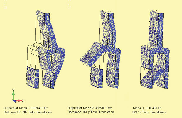Fig. 8: Fully constrained Tang with crack showing elastic modes 1-3.

Finally, the correction for the original model is to create the missing contact surface connection. It is always useful to work out what went wrong. Often this is due to tolerance definitions being too tight and hence the automatic contact creation misses out any surface pairs with a larger gap. Conversely, unwanted surface pairs can be connected in error. The normal modes check run will show these clearly.

Case Study Conclusion

Modeling errors are many and varied in practice, from the very obvious to the subtle. We all make these errors as part of every analysis project. Spotting the errors with good checking procedures and having a rational debugging approach is essential for everyone carrying out FEA. Hopefully these case studies give some ideas what to look for. In a future article we will look at other batch of case studies, all drawn from my own experiences!