Helping design and engineering professionals discover, evaluate and specify technologies and processes that shorten the design cycle and enable success.

May 2026 Special Focus: Artificial Intelligence in Design and Simulation
In this Special Focus Issue, learn about the latest developments in the integration of artificial intelligence into engineering workflows.

Design & Simulation Software Guide 2025
In this Special Issue, Digital Engineering presents its second annual guide to design and simulation software vendors.
FEA improves efficiency and minimizes component weight.
I'm an engineer with Ultra Electronics Electrics Division in Cheltenham, England, a major developer of aerospace and land military electronics applications. The division's work includes the design and manufacture of man/machine interface components, such as the yokes and control handles used in aerospace applications. The aerospace industry continually seeks to improve efficiency by minimizing component weight, and manufacturing parts from lightweight composite materials presented one potential way to do that.
Ultra Electronics sponsored my M.Sc. in FEA (finite element analysis) of composite materials at Bristol University in southwest England. I did so under the supervision of Professor Michael Wisnom, partly to investigate the use of such materials in the product range and to improve the company's knowledge of FEA systems.
Early research proved the proposed carbon- or glass-fiber epoxy composites were costly and impractical for such low-volume applications. Moreover, the materials did not lend themselves well to use in aerospace control handles without incurring a significant investment. Nonetheless, I decided to use the carbon-fiber epoxy analysis as the basis for my dissertation. My analysis experiences led to this article as well. The software I used for analysis was COSMOSDesignSTAR and COSMOSM from the SRAC of SolidWorks, supplied by CenitDesktop, an integrator and reseller of collaborative design solutions.
For the M.Sc., I first had to determine the general nature of the forces seen in a composite control handle under the maximum load exerted by a pilot. I modeled a simple control handle shape with I-deas and imported it directly into COSMOSDesignSTAR for the preliminary analysis. I used woven glass-fiber epoxy composites in this example, because their isotropic material properties enabled fast and easy modeling. I then performed a simple linear analysis to learn the nature of the stresses within the control handle. This analysis showed that interlaminar shear stress (causing the laminates to slide over each other) and interlaminar tensile stress (pulling the laminates apart) were present on the curved sections of the control handle. Those forces interact to a greater or lesser degree depending on the geometry of the curvature.
Figure 1: "Hump Back Bridge" specimens used for the finite element and experimental analysis. In this case, Y = 150mm, R = 7.5mm, and L varied between 9mm and 89mm to provide varying shear to interlaminar stress ratios.
Although the interaction of interlaminar tensile and shear stresses has received little attention and looked interesting for further study, it proved to be difficult to design a test sample that fitted a standard tensionometer to vary the interaction between the two types of stresses accurately. These studies also indicated that, in most cases, interlaminar stresses tend to dominate the failure of a composite. So, I designed a test sample that caused this failure mode to occur first.
Following on from a series of studies previously carried out at Bristol University, I used a type of laminate test specimen that cause interlaminar tensile failure (see Figure 1, above). Due to the limits of the test sample, I changed the focus of my study from the interaction between shear and interlaminar stress to the through-thickness failure of HexPly Unidirectional Carbon Prepreg (AS4 Fiber), a unidirectional carbon-fiber epoxy composite. Because all its fibers align in the same direction, this material has exceptional strength when loaded along the axis of the fibers but can be very weak in the other material directions. By varying L in Figure 1 between 9mm and 89mm I found different ratios of shear to interlaminar stress, but this only subtly affected the stress distribution around the test radius.
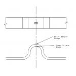 |
| Figure 2: Strain gauge location on the test specimen. Click image to enlarge. |
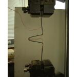 |
| Figure 3: Large test specimen immediately before interlaminar failure.Click image to enlarge. |
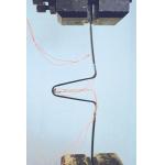 |
| Figure 3b: Close-up of the large test specimen immediately before interlaminar failure. Click image to enlarge. |
From previous studies, I knew that the stresses across the width of the specimen would be very low, allowing me to use 2D plane stress elements. For this part of the analysis, COSMOSDesignSTAR was no longer appropriate as it did not allow me to model the material properties of the composite accurately. I used the local element coordinate system in COSMOSM, and entered properties for each of the material directions. This made sure the behavior of the FE model was as close as possible to the physical test samples. It was also very important to accurately model the dimensions of the sample that have the greatest effect on the result. I learned that modeling the sample thickness as 3mm instead of the measured 2.88mm thickness varied the calculated results by up to 13% due to the cubic relationship between material thickness and stiffness.
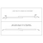
To reduce the analysis time, I used symmetry constraints along the beam centerline and fine elements only in the area of interest. I first performed a linear static analysis to verify this model and provide a useful comparison to later nonlinear analyses. As expected, the model showed considerable deformation and confirmed the need to perform nonlinear analysis.
 |
| Figure 4: Schematic illustration of the lap jointed strips. Click image to enlarge. |
After discussions with my supervisor at Bristol University, I ran a series of tests modeled with the simple isotropic materials in COSMOSDesignSTAR. My first theory examined the nature of the bending moment seen at the end of the sample, where it is "clamped" in place by the tensionometer. I thought that the magnitude of the bending moment at that point might indicate whether the model behaved in a linear or nonlinear manner. This concept can be visualized by considering two strips of material bonded together to form a lap joint, as shown in Figure 4 (above).
In linear analysis of the model, the software assumes that the deflection of the beam will not reduce the bending moment and that the offset loads will create an equal and opposite bending moment at the end of the beam. In contrast, nonlinear analysis will account for the deflection of the beam, and the resulting deformation will align the loads such that no couple is created.
; "Figure 5: simple beam showing the loads and restraints. click image to enlarge.") |
| Figure 5: Simple beam showing the loads and restraints. Click image to enlarge. |
; "Figure 6") |
| Figure 6 |
; "Figure 7") |
| Figure 7 |
Figure 6 (left) is a detail view of the loading, showing two tension loads and one downward transverse load. Click image to enlarge. Figure 7 (right) is a detail view of the constraints showing the lower 3-axis displacement constraint and the upper X-axis constraint. This allows the moment at the root of the cantilever to be calculated by multiplying the thickness of the beam with the X-axis reaction force of the upper constraint. Click on images to enlarge.
I then ran both linear and nonlinear analyses on the models and plotted the bending moment at the root of the cantilever for various magnitudes of applied loads. I could see that the FE model was behaving as it should—giving significantly lower values of bending moment, even with reasonably small beam displacements. In the case of the nonlinear analysis, the beam deflects incrementally and the axial load at the end of the beam tends to counteract the bending moment caused by the downward transverse load. The linear analysis, on the other hand, assumes that the loads remain in place and the axial load doesn't affect the bending moment of the beam in any way. Thus, the bending moment at the root is correspondingly higher on the linear analysis than the nonlinear analysis.
Now that I was sure the analysis worked correctly, I did a detailed check of all of the input properties of the models that had shown the same results for both linear and nonlinear analyses. I soon discovered that the element type used for all of the analyses had been set to "small element displacement formulation" and not the required "large element displacement formulation" stipulated in the CenitDesktop tutorial notes. By changing this variable and re-running all of the analyses I achieved FE strain results within 5% of the measured strain gauge values from the experiment. The stress results obtained are shown in Figures 8 through 10 (below).
; "Figure 8") |
| Figure 8 |
; "Figure 9") |
| Figure 9 |
Axial stress plots as shown in Figure 8 (left) are used to assist in the calculation of the strain results. A shear stress plot at the point of failure is shown in Figure 9 (right). Click on images to enlarge.
Apart from providing an important learning opportunity during the completion of my M.Sc., these analyses also highlighted factors that can affect the outcome of an FE analysis on a structure dramatically, especially a structure subjected to large deflections. Without the additional experimental work, along with an understanding of how nonlinear analyses behave, the results gained from FEA would have been significantly off the mark in terms of the stress and strain results obtained.
; "Figure 10: interlaminar tensile stresses at the point of failure of the specimen. click on image to enlarge.") |
| Figure 10: Interlaminar tensile stresses at the point of failure of the specimen. Click on image to enlarge. |
CenitDesktop
Oxford, England
COSMOSDesignSTAR, COSMOSM
SRAC Division SolidWorks Corp.
Santa Monica, CA
I-deas
UGS Corp.
Plano, TX
Ultra Electronics Electrics Division
Cheltenham, Gloucestershire, England

DE's editors contribute news and new product announcements to Digital Engineering. Press releases may be sent to them via [email protected].
Follow DEJoin over 90,000 engineering professionals who get fresh engineering news as soon as it is published.


About Us · Contact Us · Editorial Team · Advertising · Privacy Policy · Subscriber Services · © 2026 Digital Engineering 24/7 · Peerless Media
;)