Simpson's Rule

By Fred C. Jensen

Many consider DiVinci one of the greatest machine designers. His accomplishments were the result of combining his talents with the tools of the day. Imagine the potential of today’s engineers with the many tools we have available. 

The tip from the trade in this article is the use of Simpson’s Rule.  Finding the area under a curve is simplified using desktop computer tools, MCAD software, and spreadsheet programs. If you can draw the function, you can integrate it. Just take your MCAD drawing and use the property command to measure the area.

Knowing the area under a functional curve can lead to determining sectional properties of areas, then weight and mass properties of volumes, and finally physical functional properties. Almost any physical function that can be defined by amplitudes taken at regular intervals is solvable using numerical integration techniques. Applications for numerical integration include but are not limited to:

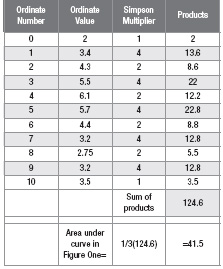
Figure 1: Simpson’s Rule is an easy-to-use and reliable method for solving numerical integrations.

a.) Calculating static and dynamic reaction forces on areas and volumes. One example would be the calculation of pressure-volume work done by a piston:

Work1-2 =  Pressure d(Volume)

b.) Solving buoyancy and stability problems when designing a new marine vessel. Examples of the use of Simpson’s rule in this discipline include the calculation of a vessel’s displacement, total wetted surface area, and the calculation of the longitudinal center of buoyancy of the hull. 

c.) Calculating the average power over an integral number of cycles of voltages and current. For example:

Average Power =  1/T    Voltage(t) current(t) d(t)

In mathematics, the most widely used solutions for the described class of numerical integration problems include the Trapezoidal Rule, Gauss Quadrature, and Simpson’s Rule. Gauss Quadrature is probably the most accurate method, but for most engineering solutions, I have found that the Simpson’s Rule is a reliable method and the easiest to use.¹

Figure 1 shows the key elements of Simpson’s Rule. To begin the process, one must collect a data stream of ordinate values at a constant interval.  We will call these ordinate values Y0, Y1, Y2, … Y10, and the constant interval, Delta X. 

Following Simpson’s Rule, one must only work with an even number of these equal distant steps. We show 10 steps in Figure 1, but this could be 6, 8, or 12 depending on the accuracy required and the type of function under study. The ordinate values are then inserted into a table, either a virtual spreadsheet table (above), or an actual paper table. Multiply each ordinate value by its Simpson multiplier. This multiplier is simply the number one for each of the two end values of the function and an alternating constant of four and two for the other values in the body of the spreadsheet table. Hence the requirement for an even number of steps. The Simpson products are simply added together and their sum multiplied by the step size, Delta X divided by three. This gives the desired area under the curve or the integral of the function Y.^{2, 3}

Volumes can also be calculated, if the ordinate values are themselves sectional areas of a 3D shape taken at regular intervals. Now that is an elegant and practical method to integrate complex functions without the need to use integral tables.³

References:
(1)  “Numerical Methods”, by Robert Hornbeck, Quantum Publishers Inc., New York, 1975, Chapter 8.2 Simpson’s Rule, pages 148-157.
(2)  “Advanced Engineering Mathematics”, by Dr. Erwin Kreyszig, Professor of Mathematics Ohio State University, John Wiley & Sons, 1979, Equation 4 Simpson’s Rule, page 787.“Principles of Yacht Design”, Second Edition, by Lars Larsson and Rolf Eliasson, International Marine, Camden, Maine, 2000, Figure 4.1, Use of Simpson’s Rule in Hydrostatics and Stability Problems, pages 30-39.

Fred C. Jensen is the director of engineering at Patriot Engineering Company in Chagrin Falls,OH. To send feedback on this toolbox tip, e-mail [email protected].