Topology Optimization

In parts 1 and 2 of this article, I dive deeper into the background of topology optimization and attempt to give insight into what controls we can exert on the process to improve the relevance to our design goals.

Fig. 1 shows a typical topology optimization analysis, based on the geometry, materials and loading definition given in the GE/GRABCAD challenge (1,2). Disclaimer: My version is not a contender.

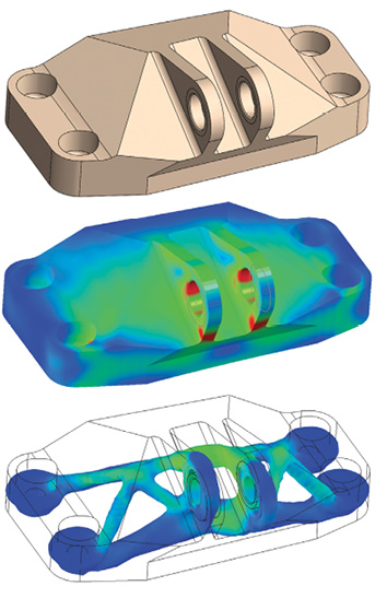Fig. 1: (a) top, initial design space. (b) middle, initial analysis. (c) bottom, final analysis.

I do recommend trying the GE/GRABCAD challenge as your own benchmarking exercise. The specification, initial geometry and full set of 638(!) results are available online.1 Various assessment papers also have been written that critique the winning designs from structural and manufacturing perspectives.

The basic idea behind topology optimization is to define a design space and mesh that with a regular array of elements. In some cases, this will be an arbitrary 3D or 2D space; in other cases, as shown in Fig. 1(a), the mesh will follow an initial scheme. We will look at the implications of this distinction in part 2. The boundary conditions and loading are defined as normal in a finite element analysis (FEA) solution, and analysis starts with the full design space as shown in Fig. 1(b). Material is progressively removed using a target volume reduction until a final iteration is completed, as shown in Fig. 1(c). The final design is assumed to be optimized to a defined level of efficiency at that target volume.

Topology Optimization Methods

Fig. 2 shows the general concept schematically. Element i is a typical element within the design space.

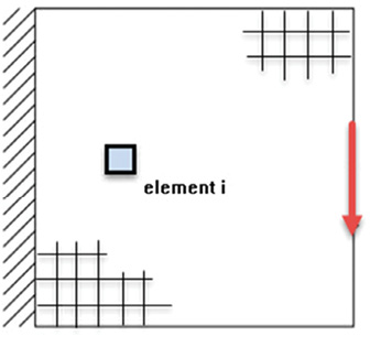Fig. 2: A schematic of FEA topology optimization.

An initial finite element analysis of this component will give a distribution of internal stress and deflection. Topology optimization seeks to improve the efficiency of the configuration by removing material based on these FEA responses. Intuitively, we could do the job manually by starting to remove material that had a very low stress level. This type of approach is called an optimality criteria method. It is based on a heuristic idea—something that looks like a good approach from an engineering point of view. A formal implementation is called fully stressed design (FSD). It is easy to implement and computationally cheap. Unfortunately, FSD does not work so well with multiple load paths, as found in most typical structures. Attempting to set all regions of the structure to very high stresses is not a realistic goal. FSD is sometimes used in a mixed strategy in combination with more sophisticated optimization objectives, such as minimizing strain energy.

Minimizing the strain energy also can be described as minimizing the compliance. Compliance is defined as the distributed force multiplied by displacement summation. Anything that minimizes the displacement distribution will maximize stiffness. Minimizing strain energy, maximizing stiffness or minimizing compliance are very closely linked concepts. All of these are global targets or objectives in that they are applied to the overall structure.

So how do we remove material from the mesh? In an FEA analysis it is efficient to keep the mesh constant throughout a series of model configuration changes. The assembly of element stiffness matrices into a system stiffness matrix at each iteration is just a scaling process on local element stiffness values. Elements aren’t deleted, but instead scaled down toward a small stiffness limit. The stiffness terms don’t quite go to 0.0, as this would give singularities.

Historically there have been two main approaches: The evolutionary methods (evolutionary structural organization [ESO] and bidirectional ESO [BESO]) aim to provide a “hard element kill” approach. This means element i is either present, with full stiffness, or effectively eliminated, with a very low stiffness. Alternatively, the penalty-driven method (SIMP) is described as a “soft kill” method and allows a gradation of stiffness range between the full value and a very low value. Other methods are available, but I am going to focus on the SIMP method in this article.

The SIMP Method

The full title of the SIMP method is “solid isotropic microstructure with penalization.” That is a bit of a mouthful, but we will attempt to break it down. The term “microstructure” is included in the title because early work looked at developing material systems that were porous and made up of voids and material in various distributions. Using this approach, anisotropic materials such as foams, lattices and composites could be defined. This work has evolved in many interesting directions, including microstructure forms for lattice-type structures in additive manufacturing. However, if the requirement is to work with conventional materials, then “solid isotropic” representation is required.

As mentioned, stiffness will be allowed to vary throughout the mesh, between initial value and close to 0.0. The design variables are defined per element, not as the stiffness, but as a normalized value for density. The stiffness is assumed to be directly scaled by the density value. The term “density” is a little confusing because the design variables are normalized values between 1.0 and 0.0.

So where does the “penalization” term originate? If a structure could develop any value of density between 1.0 (black) and 0.0 (white), we would get very large areas of “gray” material. Gray areas are not physically meaningful for a solid isotropic material. We need to cluster distributions of density toward 1.0 representing the parent material, or 0.0 representing a void. The approach taken in SIMP is to penalize any density that is in the gray region. Fig. 3 shows the penalty function used. The density is adjusted from its nominal value with a bias toward the extremes of 0.0 or 1.0. The order of the penalty function, P, is often provided as a user control. Setting P higher than 1 will give more realistic structures with less gray. Somewhere between 2 and 4 is typically used—but it is worth experimenting to see the effect.

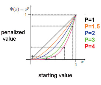Fig. 3: The penalty applied to intermediate densities.

Inherently there will always be a blurred region of density, and hence stiffness, in the SIMP method. The method does not focus on traditional boundary region features, which develop stress concentrations. The structural and, hence, stress representation is not exact at a boundary. Local stresses should be viewed as a “smeared” and averaged general indication. Similarly, the actual geometric boundary is not exactly defined. In the second part of this article I will look at these implications for stress as both a constraint and as an objective function—a possible alternative to compliance.

Mesh Dependency

Fig. 4 shows a series of models that have an increasing number of holes within them, running from 1 to 64. In each model the left-hand edge is fixed and the right-hand edge is loaded vertically, giving a shearing type response. The volume of material in each model remains the same at 65% of the volume without any holes. The resultant deflections are shown in Fig. 5.

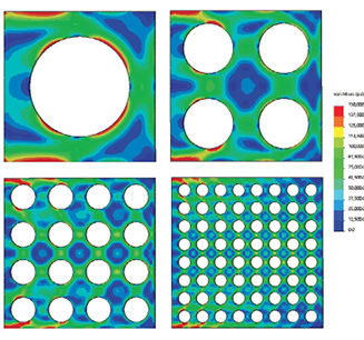Fig. 4: Component with increasing number of holes and constant volume.

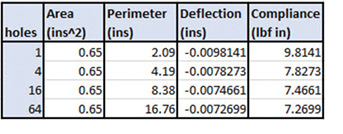Fig. 5: Variation of perimeter deflection and compliance with number of holes.

It is interesting to note that as more holes are included, the right-hand edge deflection reduces. A plot of deflection against number of holes would show a clear tendency to converge to a finite deflection value. This shows that, in the limit, we can get the stiffest possible structure at 65% of the volume by having a distribution of very tiny holes. In fact, the solution is telling us that we should be really using foam made of the parent material! If we are trying to design a structure using isotropic material then this is clearly a nonsensical result. Fig. 5 also shows that as the number of holes increases, the total perimeter is increasing. We also see that compliance is decreasing. Compliance is calculated as the applied force multiplied by the resultant deflection. Compliance is one of the most popular measures of efficiency of a structure in topology optimization.

Mesh dependency, with a tendency toward a high level of porosity, is one of the attributes of topology optimization discovered early on. For a specific optimization problem, given a target reduction in volume, the solution will depend on the element size within the mesh. A very fine mesh can drive toward a foam-like “filigree” or “fibrous” configuration. The last two typically have many very thin strands of material. A coarse mesh will constrain the optimization to a chunkier type of material distribution. It is clearly unreasonable to allow the density of the mesh to control the configuration an optimizer will deliver.

Various remedies were developed early on to reduce this effect. There are three fundamental approaches:

1. perimeter control;

2. density gradient control; and

3. density sensitivity filters.

Perimeter Control

As we can see in Figures 4 and 5, putting a limit on the perimeter to a value of 8.0 would limit the number of holes in our simple configuration to around 16. There are probably many different configurations of arbitrary shaped holes that could meet this target. But the target would clearly enforce a trend away from many small holes. One of the attractions of this method is that it is cheap to calculate and enforce this constraint in the optimization process. The main problem is that it is not physically meaningful as a parameter and is difficult to assign any kind of intuitive value to. A mathematical analogy is normally used that assesses the variation in density from each element to its set of neighbors. Fig. 6 shows a simple schematic of this. Element 1 is being assessed by measuring the density jump, dp = p2-p1, to one of its neighbors, element 2. This density jump is weighted by the element edge length L. The summation of all dp * L is made for element 1. The same process continues throughout the mesh and all values are summed. A constraint is applied to this total value, hence suppressing the tendency for density change across elements. This does have the advantage of being a global constraint, but again it is difficult to come up with a good value, and quite a few experimental runs are needed to assess the influence.

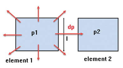Fig. 6: Perimeter control methodology.

Density Gradient Control

In this method, a physically meaningful length G, is defined as being a limit on the gradient of the density. The length G spans an arbitrary number of elements. Fig. 7(a) shows the idea schematically. Because the maximum density is 1.0 and the minimum is 0.0, then the steepest gradient is shown acting over length G. This means we are forcing the material distribution to clump together over the distance 2G, as shown—hence, this gives an effective minimum member size. In practice, because the penalty is applied to intermediate densities during iteration steps, the distribution will migrate to that shown in Fig. 7(b).

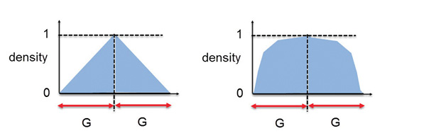Fig. 7: (a) left, density gradient control before penalty application. (b) right, after application.

In practice, more sophisticated variations are used within the optimizers, as it would be expensive to apply the huge number of constraint equations that this implies. However, the basic principle remains.

Density Sensitivity Filters

These methods use the sensitivity of the optimization responses. As the density of an element is changed, then the global compliance will change slightly. This is the sensitivity that is being used. Each element in the mesh in turn becomes a target. A fixed distance r is defined around each target element, as shown in Fig. 8. From the target to the perimeter of the circle with radius r, all surrounding element sensitivities are forced to follow a linear decrease to a value of 0.0 at the perimeter. The effect of this is to eliminate any voids within the area or volume defined by r and to enforce a “gray” type of distribution of decreasing density. However, because the overall optimization task is iterative, the penalty distribution method will rapidly migrate this distribution toward a sharper distinction between material and nonmaterial (density 1.0 and density 0.0, respectively). It will thus suppress fibrous or filigree type configurations with a width less than 2r.

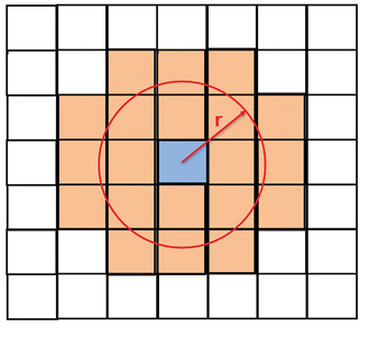Fig. 8: Density sensitivity filter method.

Checkerboarding

There is a tendency for elements to mesh together into a pattern that is similar to a checkerboard, as shown in Fig. 9. Alternating elements are connected only at the corner nodes, leaving voids between. For many types of elements, this is a stable configuration that does not cause any problems with the FEA solution. It is also a physically meaningless solution, but as in the case of the foam-like solutions seen earlier, it is numerically a relatively stiff solution. It is in fact stiffer than any equivalent “sensible” material distribution. So, it will minimize compliance and be very attractive as a solution to the Optimizer.

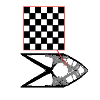Fig. 9: Typical checkerboarding result.

Various ways have been developed to suppress this effect. The mesh dependency control methods described earlier will tend to minimize the checkerboarding effect. However, relying only on these controls would mean that thin member solutions would always be suppressed, unless the controlling distance was set very close to the element size. More specifically, checkerboarding controls look directly at the connectivity logic in a group or patch of elements. This is shown schematically in Fig. 10.

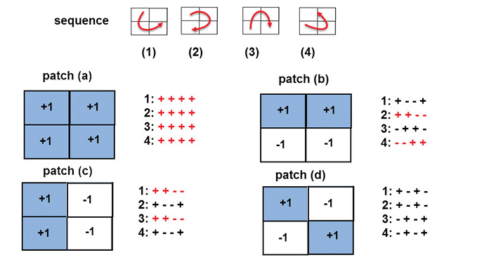Fig. 10: Connectivity logic assessment in checkerboarding.

A patch of four elements can have one of four configurations as shown by patch (a) through patch (d) in Fig. 10. A set of four sequences (1) through (4), moving between these elements is shown in the upper sketch. A pattern describes how the elements flip between non-zero density, (+1) and zero density (-1). The various patterns are shown to the right of the patch configurations. A monotonic sequence (colored red) is defined as one that stays constant, increases or decreases. An oscillating sequence (colored black) flips between positive and negative. All patches except patch (d) show at least one example of a monotonic pattern. So, each patch of elements within the mesh is searched for at least one monotonic sequence. If none are found, then there is a checkerboard patch present; this can be eliminated by smearing effective material over all four elements in the patch.

There are quite a few variations on this technique.

The basic numerical approach behind the SIMP method has been shown, together with provisions for mesh independency and checkerboarding. In part 2 we will look at the alternative objectives and constraints available. We will also see how manufacturing constraints are enforced, and derive some general guidelines for controlling topology optimization. DE

Tony Abbey works as training manager for NAFEMS, responsible for developing and implementing training classes, including a wide range of e-learning classes. Check out the range of courses available, including Optimization: nafems.org/e-learning.

Editor’s Note: Tony Abbey teaches live NAFEMS FEA classes in the United States, Europe and Asia. He also teaches NAFEMS e-learning classes globally. Contact him at [email protected] for details.