Stress in FEA: Part 3

Editor’s Note: Tony Abbey teaches live NAFEMS FEA classes in the U.S., Europe and Asia. He also teaches NAFEMS e-learning classes globally. Contact [email protected] for details.

In part one of this series, we looked at the fundamentals of forces and stresses. In part two of this series, we looked at directional stresses in the XY plane of the structure shown in Fig. 1. It is a cross brace, supported at the left-hand edge by two lugs and loaded at the right-hand edge through two additional lugs. The structure is sitting in the global XY plane.

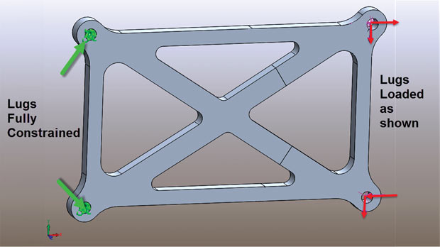Fig. 1. Cross brace structure showing constraint and loading set up.

In this article we are going to look at two further types of stress: principal stress and Von Mises stress.

Principal FEA Stresses

In the previous article we focused on the Cartesian stresses SX, SY and SXY. We saw that for a particular coordinate system these were the stresses in the local X, Y direction and XY plane, respectively. We rotated the stress system from the basic XY coordinate system to two other coordinate systems to look at local ‘cut’ directions. In fact, we can rotate the stress state to any coordinate system we want. It is important to realize that we are always describing the same stress state, but just viewing it from a different angle.

Fig. 2 shows the equations that can be used to calculate the stress in a local coordinate system, by using a rotation through an angle. These are exactly the same equations that will be used by your post processor to flip from one coordinate system to another. You may remember having to plot these transformations by hand using the Mohr’s circle construction. It was very convenient to do it this way before electronic calculators came along. (I will take a look at Mohr’s circle in more detail in a later article).

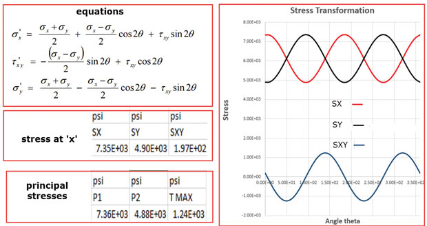Fig. 2. 2D stress transformations

We’re going to pick a datum point on the structure, adjacent to the top right hand corner lug. This is shown in Fig. 3, where we also see the stress contours for Cartesian SX, SY and SXY stresses. The stress values at the datum point are shown in the Fig. 2, labeled “stresses at x.” If we substitute these values into the equation in Fig. 2 then we can plot the variation stress at the datum point as we rotate around all the possible local coordinate systems. The resulting plot is shown in Fig. 2.

Looking at Fig. 2 we can see that the stress varies in a cyclic manner as we rotate around the full 360°. There are some other interesting rotation angles we can see in this plot. The direct stresses SX and SY peak together at the same rotation angle. At this rotation angle the shear stress SXY drops to zero. The biggest and smallest direct stresses we find at this particular angle are called the principal stresses. The values are shown in Fig. 2. In a 2D stress state, these are labeled as P1 and P2. There is a further angle where the shear stress SXY is a maximum. This value is called maximum shear stress. We actually have a 3D stress state in this structure, although the dominant responses are in the XY plane. For a 3D stress state the principal stresses become P1, P2 and P3. Usually, P2 is a very small stress and we are only concerned with the values of P1 and P3. The menu selection for 3D contour stress plotting usually contains P1 and P3 principal stress components.

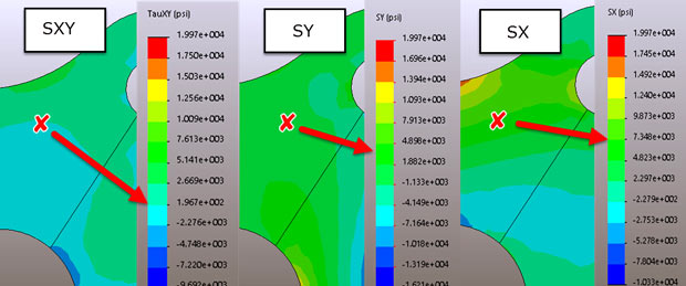Fig. 3. Stresses at the datum point x

Fig. 4 shows stress contour plot of the maximum principal stress P1. This is a useful way of seeing the biggest tensile stress flow direction. I have clipped the contour at around the zero stress line so tensile stresses dominate. The gray zone contains either very small tensile stresses, or compressive stresses. If the P1 stress level is compressive then it means that the stress state is always compressive, no matter what angle we choose for a local coordinate system. So, a quick eyeball of this structure shows that the top member is totally in tension throughout its depth. The transverse member (top left to bottom right) has a small tensile stress flow. The right hand vertical member has localized tensile regions, which are clearly the positive side of the bending distribution. We plotted this bending distribution in the last article.

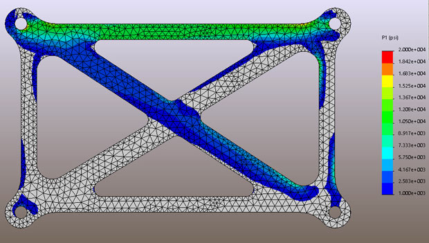Fig. 4. P1 stress distribution for the overall structure

The contour plot in Fig. 5 shows the P3 distribution through the structure. Again, I have clipped this plot so only compressive stresses are shown. By definition, any region that has a minimum (most negative) P3 stress that is positive, must be a tension dominated region. These regions are now in the grayed out zone. The two plots in Figs. 4 and 5 are complementary: They show, respectively, the zones of tensile and compressive dominated structure.

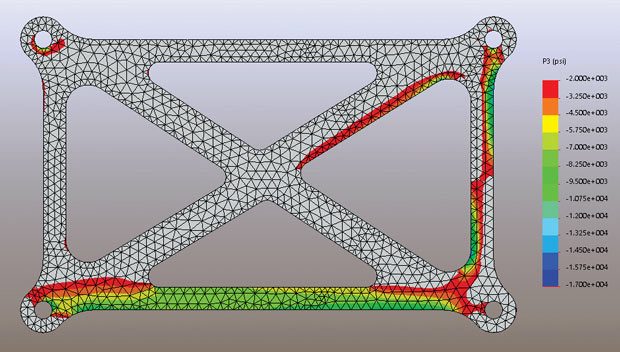Fig. 5. P3 stress distribution for the overall structure

Figs. 6 and 7 show, respectively, contours of maximum and minimum principal stresses P1 and P3 for the local lug region. The insert XY graphs show tensile principal stress running along the top lug fillet radius and compressive principal stresses running around the side fillet radius. These two figures illustrate how useful the principal stresses are. By definition, along a free surface, the stresses must be tangential and will naturally form principal stress directions. Running a line plot along the surface will show the distribution of peak stress. This really is the only way that this can be visualized and it is a powerful investigation tool.

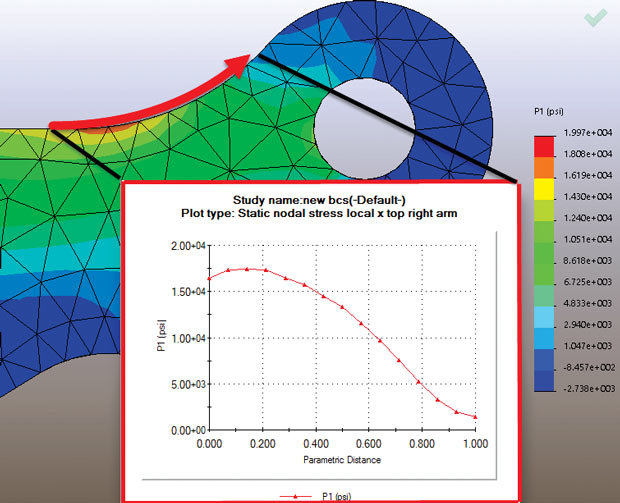Fig. 6. Tensile principal stress running around the top lug fillet radius

I find that contour plotting of principal stresses segregated into tensile and compressive dominant regions is a useful approach. However, the more normal way of presenting principle stresses is via a vector plot. Fig. 8 shows a vector plot of the P1 principal stresses running around the lug region. The tensile dominated regions are shown clearly, however the compressive dominated regions “fizzle out,” with very small values of P1. Fig. 9 shows the complementary plot of P3 principal stresses and the compressive zone around the fillets can be seen very clearly. Again, the small smaller values of P3 associated with the tensile regions are “fizzling out.”

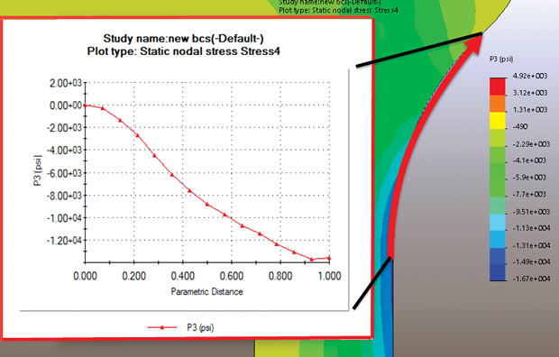Fig. 7. Compressive principal stress running around the side lug fillet radius

In this particular post-processor, we plot P1 and P3 vectors separately as shown. Other post-processors will allow an overlay of P1 and P3 vectors perpendicular to each other. Both are equally valid representations; some analysts prefer two plots that distinguish P1 and P3 more clearly, some prefer to have a combined plot. Whichever we use, there is no doubt that the vector plots give a good representation of the flow of the stress. This is one of the most useful aspects of principal stress plotting. The main difficulty is that the small P1 stresses in a compressive zone and the corresponding larger P3 values in the compressive zone can also spoil the visualization (what I have described as “fizzling out”). I prefer to segregate the two plots and control the clipping of the vector values carefully to aid visualization.

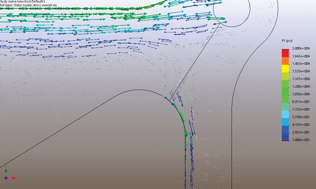Fig. 8. P1 principal tensile stresses running around the fillet radii of the lug region

P1 principal stresses are useful when considering fatigue and fracture. We may not be completely sure of the relative orientation of a stress flow and a crack. The most damaging orientation will be at 90°. We can use the P1 principal stress as an upper bound estimate for the biggest tensile stress we can ever see across the crack in this region. In a similar way, a critical compressive stress can be found by using the P3 principal stress. In the region prone to buckling it can be difficult to assess the relative orientation between the slenderest direction (which is most prone to buckling) and the dominating compressive stress. By assuming a value P3 for stress, then we have defined the worst case.

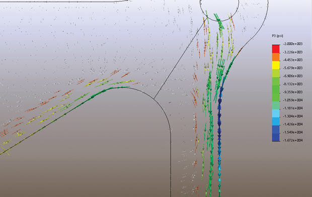Fig. 9. P3 principal compressive stresses flowing around the fillet radii of the lug region

Von Mises Stress

Finally, we come to the most common stress plot in normal use and you may wonder why I have left it for last. The reason: It is difficult to explain what von Mises stress means unless we have a good understanding of the contributing component stresses. The von Mises stress equation for 2D is:

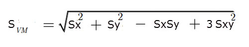Fig. 10. von Mises stress equation for 2D stresses.

We do actually have a 3D state, but this component’s response is predominately in-plane. I have ignored the SZ, SXZ and SYZ through thickness stresses for this article. Looking at the equation in Fig.10 we can see that each stress component is squared and there is an interaction term between SX and SY. The shear stress SXY is factored by three. Imagine a stress state with SY and SXY at zero; the von Mises stress then equals SX. The same argument applies to pure SY stress. However, if we have a pure shear stress, then the von Mises stress is factored by square root of 3. This last observation agrees with the general case where the shear yield stress is lower than tensile yield stress. I will go into more detail about yield criteria, such as Von Mises yield, in a later article.

Fig. 10 shows the von Mises stress distribution for the overall component. We see that there are three or four regions of high stress. This is the big advantage of the von Mises stress plot; it allows us to identify problem areas. The von Mises stress level can be compared directly to tensile yield stress and gives a good indication of margins over potential plastic response.

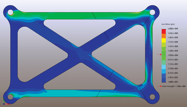Fig. 11. von Mises stress for the overall structure

On the other hand, the main disadvantage of the von Mises stress plot is that we are encapsulating all the stress components into one scalar value. If we only plot von Mises stress, then we miss two important factors and cannot tell whether the stress state is tensile or compressive. We do not know whether the stress state is direct stress dominated or shear stress dominated.

Fig. 11 shows the lug region with von Mises stress contours. The stress concentrations can be seen, but clearly we need to differentiate between tension and compression. The differential between tension and compression is important in fatigue analysis—we need to know whether we are in a beneficial compressive stress state or an aggressive tensile stress state. For relatively thin or slender structures we are also concerned that the compressive stress state may induce local buckling. By default, a linear static analysis is not going to pick this up, so we need to inspect carefully for any suspect regions. Finally, in many ways, shear is a more damaging stress state than direct stresses, so it is as well to be aware of its presence.

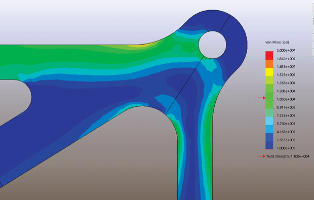Fig. 12. Von Mises stress for top right corner

A Recipe for FEA Stress Investigation

In summary, we have three main types of stress that we can use for investigation: Cartesian stresses, principal stresses and von Mises stress. I normally run through them in the following order when post-processing a finite element analysis model.

1. Von Mises stress. This is checked as an overall indicator of stress distribution and stress concentration location. The margins over yield are identified.
2. Cartesian stresses. Regions flagged up by the von Mises stress plot are broken out into separate Cartesian stress plots SX, SY and SXY. This is fairly straightforward for 2D dominated responses as shown in this article. However, a 3D response may require an approximation to in-plane and through thickness directions to aid visualization. Transformation into convenient local coordinate systems, to align with the structural with the local structural configuration, will help visualization. The objective of the Cartesian stress plots is to show which stress types dominate.
3. Principal stresses. Contour and vector plots of maximum and minimum principal stress are very useful to give a sense of the stress flow. The stress values can also be used where worst-case compressive or tensile stresses, or maximum shear stresses are needed.

It is quite a learning curve to go on from the usual von Mises contour plot to more in-depth usage of Cartesian and principal stresses and local coordinate systems also add a level of complexity. However, if you are serious about understanding the nature the stress inherent in components, then it is worthwhile to investigate these techniques. Typically, this will be an exercise on two fronts; becoming comfortable with the physics of stress states and also with the advanced tools found in the post-processor interface.