Stress in Finite Element Analysis: Part 2

Editor’s Note: Tony Abbey teaches live NAFEMS FEA classes in the U.S., Europe and Asia. He also teaches NAFEMS e-learning classes globally. Contact [email protected] for details.

In part one of this series, we looked at the fundamentals of forces and stresses. In this month’s article we are going to look at how we use these stresses in a practical example. The structure we shall use is shown in Fig. 1. It is a cross brace, supported at the left-hand edge by two lugs and loaded at the right-hand edge through two lugs. It is sitting in the global XY plane.

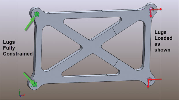Fig. 1: Cross brace structure showing constraint and loading set up.

We are going to investigate the stresses throughout the structure and relate them to the fundamental ideas we looked at in the last article.

Last time we established the meaning of the direct normal stresses at a point and these were labeled as SXX, SYY and SZZ. The structure we have is three-dimensional, but the loading and constraint system gives a stress distribution acting mainly in the global XY plane. We can ignore the stresses through thickness i.e. the SZZ terms. We will abbreviate the normal stress terms to SX and SY.

Fig. 2 shows a plot of the stresses in the X direction, the SX stresses, throughout the structure. Many of you are probably wondering: At this stage why not just plot Von Mises stresses? I will come to that in the next article, but I want to progress in a logical way, building up our knowledge of stress types.

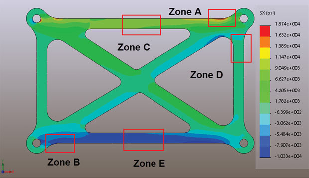Fig. 2: Zones of interest A through E and the SX stress distribution.

Searching for Stresses

The stress distribution in Fig. 2 doesn’t give us a good overall picture of what’s happening in the component. However, some of the zones of interest are aligned with the global X direction and that makes it convenient to look at stresses in those regions. If we think of this structure as a space frame, we can picture an overall bending response, with tension in the top ligament and compression in the bottom ligament. Looking at zone C, it must be a tensile load path. The X direction stresses are useful here.

Fig. 3 shows the distribution of X direction stresses local to zone C. The stress contours have been clipped to the local regional values. Inspecting the contours shows a variation in axial loading from almost pure membrane tension loading to membrane plus bending loading. The stresses could be easily summated over the cross-section to give the Fx axial force and Mz bending moment at these two stations. Many post processors are able to do free body diagram section cuts like this automatically. It is well worth investigating these and comparing the stress distributions with resultant forces and moments.

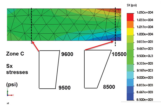Fig. 3: Zone C X direction stresses showing membrane and bending distributions.

If we set up a simple beam model of this cross brace structure, we should be able to get bending moment and shear force diagrams, which would give similar values to those found here.

We can carry out a similar exercise on the lower horizontal at zone E. Intuitively we know that this is going to be a compression loaded member and the X direction axial stresses confirm that, as shown in Fig. 4. Again, we can see a buildup of bending moment as we move toward the right-hand lug.

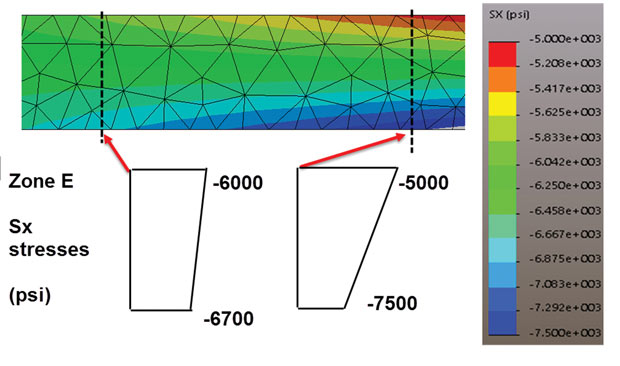Fig. 4: Zone E Axial X direction stresses showing membrane and bending distribution.

Where else on the X direction stresses of any use in predicting the behavior of the component? Reviewing Fig. 2, we can see that the only areas that may be of interest are zones A and B. These look like the most highly stressed regions, but the X direction stresses alone are not giving us the full story.

The cross braces and vertical members are not aligned with the global X direction, so the X direction stresses are not much use here. However, if we use the same logic, we can look at the Y direction stresses as being meaningful for the vertically orientated members. Fig. 5 shows the Y direction stresses plotted on the structure. Now zone D is showing up clearly as an area of interest. There is a similar region at the bottom of this vertical member, with a reversed stress sense.

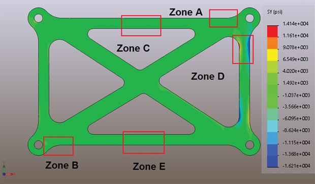Fig. 5: Vertical Y direction stresses throughout structure.

We can zoom into zone D, plotting the Y direction stresses, and clipping the values to the local region maximum and minimum. The result is shown in Fig. 6 and clearly indicates a small compressive load path with a relatively large bending moment. This bending moment in the vertical member is complementary to the bending moment we can see in the horizontal member at zone A. We need to look at Fig. 2 to see this.

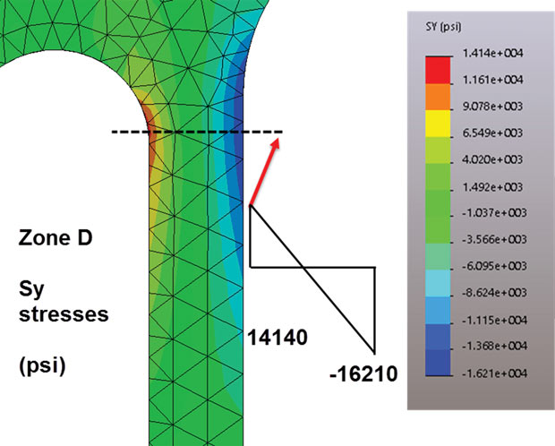Fig. 6: Vertical Y direction stresses in zone D showing compressive membrane and bending behavior.

As mentioned earlier, there is a reversed bending moment just above the bottom lug in this member. The design of the lugs is not very good as the line of loading action is offset from all the bracing members. This is introducing large kick moments. It is also interesting to note that there is a low compressive axial load in the right-hand vertical member. Both top and bottom lug are loaded in a downward sense, rather than just the bottom lug.

Local Coordinate Systems

So far we have investigated global directional stresses SX and SY. This has given a good indication of the response of the horizontal and vertical members. However, what happens if we want to investigate the diagonal cross members at Zones F and G? Global stresses are useless to us here, as it is impossible to picture the stresses and the resultant forces.

The answer to this is to set up local stress coordinate systems. Almost every FEA (finite element analysis) postprocessor will be able to transform stresses from the basic global coordinate system to any desired local coordinate system. In Fig. 7, I am plotting local X direction stresses at zone F, aligned with the bottom right-hand cross member axial direction. This requires defining the local coordinate system and then making sure the stresses are transformed into this coordinate system.

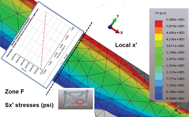Fig. 7: Local X direction stresses aligned with the cross member at Zone F, showing act axial and bending distribution.

Fig. 7 shows the net tensile axial force and bending moment distribution in both contour plot form and xy plot form.

In preparation for the xy plot, I split the geometry to form a regular face of nodes at the split face. This was done at zone F and G. This is the best way to produce accurate results at a station cut. If a virtual cut section is used instead in post-processing, it will use interpolation across what can be a very ragged set of elements. Results can be very poor.

In part one of this series we also looked at shear stresses. For this component, we can imagine the shear stresses running across the cut face, at right angles to the axial stresses. Fig. 8 shows the contour plot of the local shear stress and also an xy plot of the distribution across the section. The distribution of the xy plot shows the classic parabolic shear stress distribution across a rectangular section as we discussed before. Shear must be zero at the free edges. The value of the shear stresses and the resultant integrated force is very low.

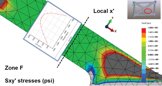Fig. 8: Local XY shear stress plotted for the bottom right cross brace at Zone F.

A second local coordinate system is used to recover local stresses in zone G, which is the upper right cross brace. Fig. 9 shows a contour plot of the local X direction stresses. Only the mesh highlighted is relevant for these directional stresses. The stresses are valid in the other parts of the structure, but the directional components are useless in attempting to understand the nature the stresses. This type of partial directional regional plot is very common in a detailed post processing report. An extreme example of this is the use of local coordinate polar plots that show radial and circumferential stresses around specific bolt holes.

Zone G is showing predominantly axial compression loads, combined with local bending. The lateral direct loading SY is also plotted, and shown to be negligible. The shear stress SXY across the section is also very low, again showing a parabolic distribution.

By inspection of Fig. 9, we see the bottom left-hand brace is also in compression, but with no local bending present.

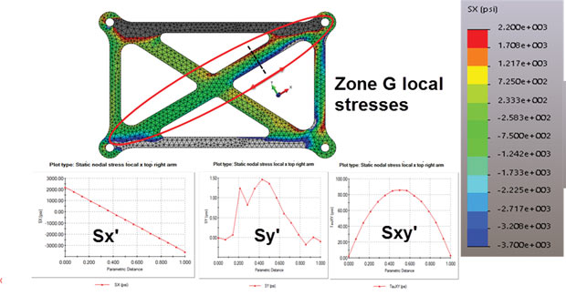Fig. 9: Zone G stress distributions; SX, SY and SXY in the local coordinate system.

Fig. 10 shows the global XY direction shear stress plotted for the complete structure. Not much can be deduced from this other than that there is a shear stress contribution at peak stress zone A.

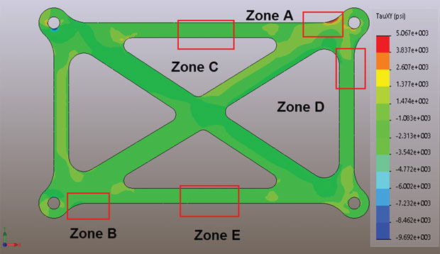Fig. 10: Global shear stress XY disparate distribution throughout the component.

Heading in the Right Direction

In summary, directional stresses are very useful in understanding the load paths within component regions. We have been able to identify the overall response of the structure by using a series of local coordinate systems. Transforming stress coordinate systems is usually a very straightforward post processing task and it is something well worth practicing. Using these transformed stresses, described as Cartesian stresses, is just part of the set of tools that we have available to understand the response of the structure.

In the next part of this series we will look at the theory behind stress transformations, which leads us onto principal stress definitions. We will discuss practical application of principal stresses.

Finally, we will look at Von Mises stress and dig a little deeper into what it means. It is tempting to only use Von Mises stress when reviewing structures. By discussing it last, I hope to show the importance of the other methods.