Linear and Nonlinear Buckling in FEA

Editor’s Note: Tony Abbey teaches live NAFEMS FEA classes in the U.S., Europe and Asia. He also teaches NAFEMS e-learning classes globally. Contact him at [email protected] for details.

Buckling occurs as an instability when a structure can no longer support the existing compressive load levels. Many structural components are sufficiently stiff that they will never suffer any form of instability. In Fig. 1 these structures are classically described as “short.” In practice it is the relationship between radius of gyration and length that is the deciding factor and hence long span girders of heavy section could easily be clear of any instability mode. This type of structure would only fail in compression by local yielding if load levels can reach that extreme.

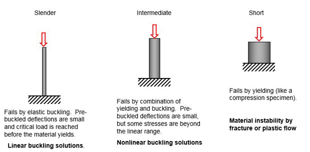Fig. 1: Classical identification of structural types and buckling response.

At the other extreme, structures that are slender could fail at load levels well below what is required to cause compressive yielding. The failing mode tends to be toward the classic Euler buckling mode. For long thin rods and struts the Euler buckling calculation can be quite accurate. The buckling here is of a bifurcation type — there is a rapid transition from axial loading response to a lateral response, which is usually catastrophic.

A very large number of structures fall into the intermediate category where the Euler buckling calculation is not very accurate and can tend to seriously overestimate the critical buckling load. The transition to instability is more gradual in this category. The structure is able to carry increasing loads, with perhaps changes in deformed shape and plasticity, until a maximum (or limit) load is reached. At this point instability occurs. This may be catastrophic, or the structure may transition to a new mode shape that can carry further load. Examples include the initial buckling of a drink can, initial buckling of a thin wing spar shear web, or the light frame of a screen door.

This article looks at various buckling calculation methods in finite element analysis (FEA).

Linear Buckling

The most basic form of buckling analysis in FEA is linear buckling. This is directly related to the classic Euler type of calculation. A small displacement of a perturbed shape is assumed in each element that induces a stress dependent stiffening effect. This adds to the linear static stiffness in the element. Imagine a guitar string tightened—the string’s total stiffness goes up and results in a higher pitch. If the string is slackened the total stiffness goes down, and the pitch corresponds. The stress dependent stiffness is now subtracting from the linear static stiffness term. This latter effect causes buckling.

In an assembly of elements in an FEA model there will be a subtle interaction between the original linear stiffness matrix and the stress dependent stiffness matrix. This is analogous to the linear stiffness matrix and the mass matrix in a normal modes analysis. The same solution method is used—an eigenvalue extraction. For a linear buckling analysis, this will find what scaling factors applied to the nominal static load will scale the stress stiffening terms to subtract sufficiently from the linear static terms to give unstable solutions.

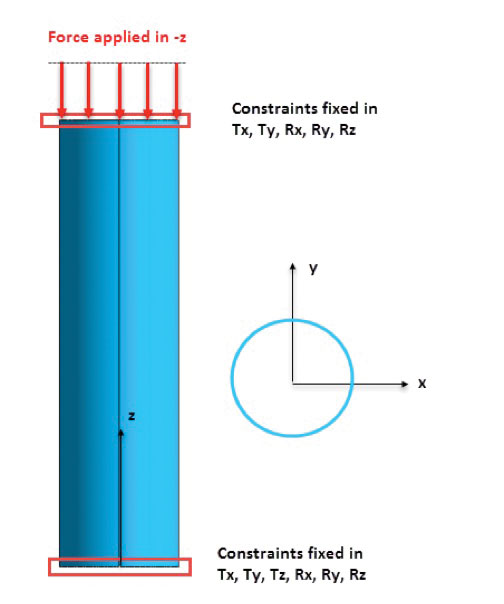Fig. 2: Typical FEA buckling analysis set up, axially loaded cylinder.

Fig. 2 shows a typical analysis setup. An axial load of a nominal 1KN is applied to the top of a thin-walled cylinder. The constraint systems are shown. A linear buckling analysis is carried out. The stress stiffening matrix and the linear static stiffness matrix are calculated in the first linear static step. In the second step the unstable roots are found using the two matrices in an eigenvalue solution. The user doesn’t have to do anything special here because all buckling solvers are “hard-wired” to do the two steps.

The result of the analysis is a table of eigenvalues as shown in Fig. 3 and a set of mode shapes, or eigenvectors. The first mode shape is shown in Fig. 4.

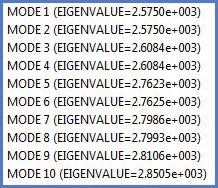Fig. 3: Table of eigenvalues.

The critical load that will cause the first buckling mode is calculated from the nominal load (1KN) multiplied by the eigenvalue (2.575E3 from Fig. 3). So the critical load is 2.575E3 KN. We can see the mode shape in Fig. 4. An important question is: Can we use the deformation values shown in the figure? The answer is a definite no. Just like a normal modes analysis, all we can get is the shape of the buckled mode. There is no meaning to the values shown in Fig. 4. The length of the cylinder is only 1.5 m, so a displacement of 0.8581 m as shown would be well beyond any sensible result. We are assuming small displacement perturbations—or shapes. We have no way of allocating displacement values.

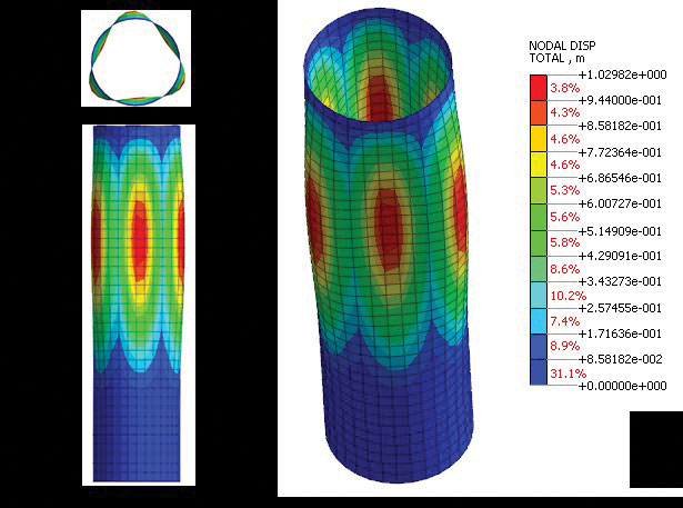Fig. 4: First eigenvalue or mode shape.

The second important question is: Can we use the stresses calculated from the mode shape and often shown in a linear buckling analysis? The answer again is a very definite no—for two reasons. The displacements are arbitrary and therefore the strains and stresses are as well. The second reason is that the mode shape is only a perturbation normal to the loading axis, so in fact does not couple with the axial load present just before the buckle. This may seem a bit surprising so I have shown the effect in Fig. 5 and Fig. 6. A connecting rod is analyzed for linear buckling and also for nonlinear buckling. We will go into nonlinear buckling shortly, but basically it allows a continuous load build up and then transition to buckling. Fig. 5 shows a pure bending distribution across the conrod in the linear buckling solution. Clearly there is no contribution from the axial loading. The stress result is meaningless. By contrast, Fig. 6 shows a transition of stress in a nonlinear analysis from purely axial just below buckling, to axial plus bending at buckling. The stresses and displacements in the nonlinear case are meaningful.

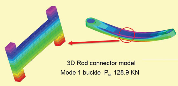Fig. 5: Linear Buckling mode shape and ‘apparent’ stresses.

Coming back to our cylinder: What do we get from the linear buckling analysis? An estimate of the critical buckling load and the likely mode shape that will result at buckling. We do not know what happens next. Will the cylinder collapse or stiffen? What will the final stresses and displacements be?  It is rather like a freeze frame photo just at the initiation of buckling—we are left in suspense.

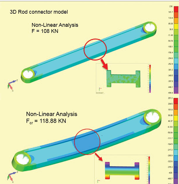Fig. 6: Nonlinear buckling showing stress transition just below and at buckling.

The information we get is very useful in design, but it is more of an indicator than a hard number. We also have to be aware that if we use linear buckling on a structure that is more like the intermediate category, then we are likely to get a non-conservative over estimate of the buckling load. We may also find the mode shape transitions very quickly into something very different.

The boundary condition assumptions for buckling are also critical. However, if the structure can be categorized as “slender” and we can show a good margin over the critical linear buckling load, then in many cases that is sufficient for design.

Fig. 7 shows the higher order modes shapes associated with eigenvalues 1 to 10. Very often the default in an FEA solver is to just have the first eigenvalue and mode shape. In fact, the study of the higher modes is useful.

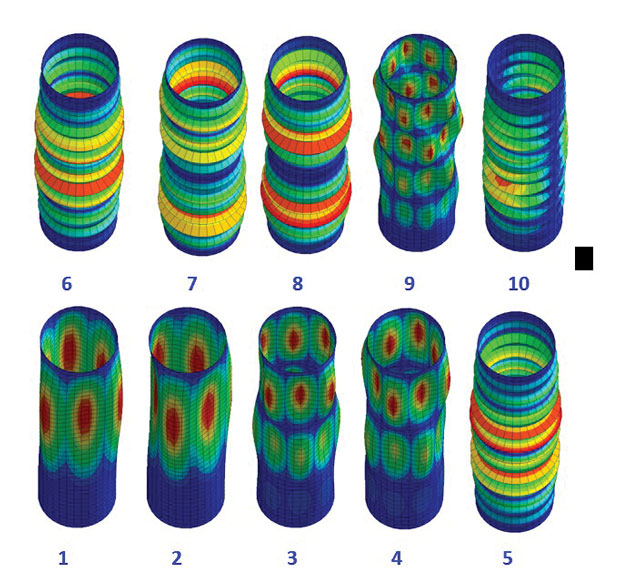Fig. 7: Cylinder buckling mode shapes 1 to 10.

We can see that mode 1 and 2 are identical and represent a repeated mode—any arbitrary axial orientation of the fundamental shape is possible. Modes 3 and 4, 5 and 6, and 7 and 8 are also repeated roots. We can also see a distinction between “dimpled” shapes that have a low number of axial lobes and “Chinese lantern” modes, which have a high number. The range of eigenvalues is also low—and actually defines critical loads of 2.57E3 to 2.85E3 KN. The implication is that any small variation in boundary condition, component detail or load eccentricity could cause any of the modes to occur. The modes are completely independent in the linear analysis; so mode 1 or 2 or 3, etc. could occur. One way to imagine this is if mode 1 and 2 pair were not possible in practice, by snubbing against adjacent components, etc., then mode 3 and 4 pair could occur.

It is important to assess the families of higher mode shapes and eigenvalues to see if any practical response implications occur.  However often there may be only one dominant first mode, with the next set of modes completely infeasible and at very high critical loads. These can be ignored.

Nonlinear Buckling Analysis

If for any reason the results of a linear buckling solution suggest the calculation is not representing the real response, then a nonlinear buckling analysis is called for. This uses a nonlinear geometric analysis to progressively evaluate the transition from stable to unstable and addresses many of the limitations we have seen in linear buckling analysis.

The DE article “Moving Into the Nonlinear World with FEA” offers more insight on nonlinear buckling analysis.

Fig. 8 shows the first attempt at a nonlinear buckling analysis. It is very disappointing as all we see is an axial shortening with no sign of buckling.

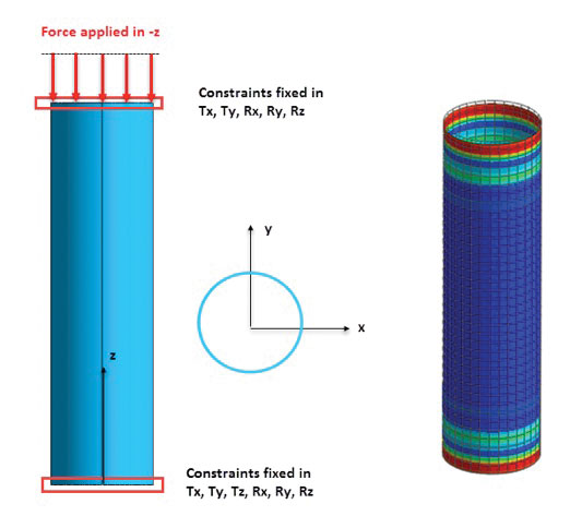Fig. 8: Initial attempt at a nonlinear buckling analysis.

This uncovers another difference between linear and nonlinear buckling. In linear buckling the small perturbations the structure may see are “hard wired” into the solution. For nonlinear analysis, the perturbations have to develop geometrically as part of the solution and are not pre-defined in any way. The theoretical solution in Fig. 8 totally ignores fundamental facts of nature. No component can be perfectly straight, have perfect constraint application or perfect load application. No material content will be absolutely homogeneous. All these factors give rise in practice to small eccentricities and variations that attract offset axial loading. This in turn starts to produce offset moments that cause further eccentricity. For a very stable real structure no buckling will occur, but for an intermediate category real structure the eccentricities will grow until instability occurs. In a real slender category structure it will happen more quickly, but probably not as abruptly as the linear Euler solution predicts.

How do we overcome this limitation? Some components and loading will have such a large natural eccentricity that the solution will find instability. However for our stubborn cylinder we have to introduce an eccentricity. There are several ways of doing this. All methods can benefit from our understanding of the linear buckling mode. The nonlinear mode may transition through this, but it is a good starting point. We can either apply a “dummy” loading to induce the mode shape, or actually distort the structure very slightly in favor of the mode shape. The first method is usually easiest, as any sympathetic load will usually work. Pressures are better than point loads as they avoid local singularities. If possible a sympathetic pressure can be applied in the same distribution as the normal displaced mode shape from the linear analysis. It can be captured as a field function and scaled to suit. It is difficult to assess what level of load to apply, but it should be a lot smaller than the main axial loading.

In the case of the cylinder, I applied a pressure over one quarter vertical strip to give a net sideways thrust. This dummy static load was set to give a deflection of 3.5e-4 m—a very small wall deflection. The best way to do this is to ramp up the dummy load as the main loading is applied, and then to ramp it down to zero until 100% main load is achieved. Alternatively, a pre-stress load case may be possible, which will not get scaled up as the main loading is increased. The setup will depend on your FEA program. If all else fails you may have to apply a small dummy load, which will increase with the main load and be there as a small “artifact” at the end.

The other alternative is to capture the linear buckling mode shape and apply this back to the structural mesh as an initial distortion. Again this can use a field function from the mode which is scaled and used as an offset, or the same thing can be done via an Excel export. Your FEA solver may well have automated ways of handling this. A word of caution here though: if you make the imperfections too big you will effectively corrugate the structure and stiffen it up. Trial and error is required.

Fig. 9 shows the results of the nonlinear buckling analysis. The cylinder configuration and the level of eccentricity assumed result in a very stable structure that resists buckling until a mode occurs, similar in nature to the linear mode. There is then a transition to a highly localized mode. The initial buckling occurs at around 63% of the linear estimate for critical load. The maximum load level achievable before the structure sees a local collapse is about 82% of the linear critical load.

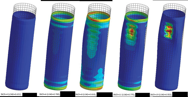Figure 9. Progressive stages in nonlinear cylinder buckling

The nonlinear method used to track the geometric instability was the Arc Length method. This is always recommended as it enables the softening response of the structure to be tracked. When a structure buckles it has less resistance to load. A real-world load controlled test would result in a runaway collapse. Alternatively, a real-world displacement controlled test would allow us to monitor the reducing load resistance. The Arc Length method permits this, even though we are applying load.

Important considerations are: What is the effective critical buckling load level and what is the post-buckling behavior? I like to use key point plots to investigate this. Fig. 10 shows a shell element identified as being a good indicator of the changing stress state as instability occurs. Membrane hoop stress is zero and axial stress is steadily increasing up to the start of instability at point A. This is a classic linear response. From A to B the hoop stress increases as the structure distorts. From B to C a second mode occurs with a further instability local to this element, the axial stress decreases as the structure softens. The overall response in Fig. 9 shows the transition to local dimpling. In fact this region would rapidly exceed yield in practice, but a linear material model has been used.

Fig. 10: Key point plot; stress response at key element

Fig. 11 shows the radial displacement response of two key nodes, one at an outward moving lobe, and one at an inward moving lobe. Corresponding points A, B and C correlate well with Fig. 10 and confirm the onset of instability.

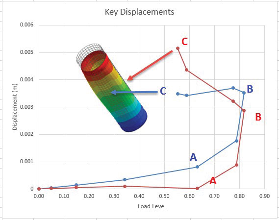Fig. 11: Key point plot; radial displacement response at key nodes.

In practice, the model should now be investigated for sensitivity to initial induced eccentricity and preferably comparing several forms of induced eccentricity. Effects of constraint and loading implications can be compared to the real-world conditions by experimenting with DOF (degrees of freedom) and using boundary spring stiffnesses. The load steps can be adjusted to give finer results closer to initial instability. Plastic behavior could also be investigated in the transition to the second instability.

Conclusion

Buckling is a critical failure condition for many classes of structure. Accurate estimates of critical load and response modes are difficult unless a structure falls well into the “slender” category. Linear solutions may suit such structures if loads and boundary conditions are carefully assessed. However for the majority of instability prone structures a full nonlinear analysis is required. This type of analysis is very sensitive to assumptions on eccentricity and boundary conditions. A methodology is required that will deal with structural softening. The key point method is recommended to help identify the onset of instability and subsequent transitional modes.