Helping design and engineering professionals discover, evaluate and specify technologies and processes that shorten the design cycle and enable success.
Alert!
Digital Engineering ceased publication on July 1, 2026. This website remains available as an archive of engineering content.
For inquiries or information, please email [email protected].

May 2026 Special Focus: Artificial Intelligence in Design and Simulation
In this Special Focus Issue, learn about the latest developments in the integration of artificial intelligence into engineering workflows.

Design & Simulation Software Guide 2025
In this Special Issue, Digital Engineering presents its second annual guide to design and simulation software vendors.
In fields such as microfluidics, medical research and the pharmaceutical industry, the precise metering of very small volumes of liquids or gases is important. This is often achieved by employing piezoelectric micropumps, which can be controlled with high precision. Mathematical modeling and numerical simulation help accelerate the optimization of such devices and thus reduce the cost of development and time to market.
Today, we will discuss how to use the COMSOL Multiphysics software to simulate a piezoelectric micropump, using an example model contributed by engineers at Veryst Engineering, a COMSOL Certified Consultant company, including Riccardo Vietri, James Ransley and Andrew Spann.
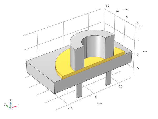
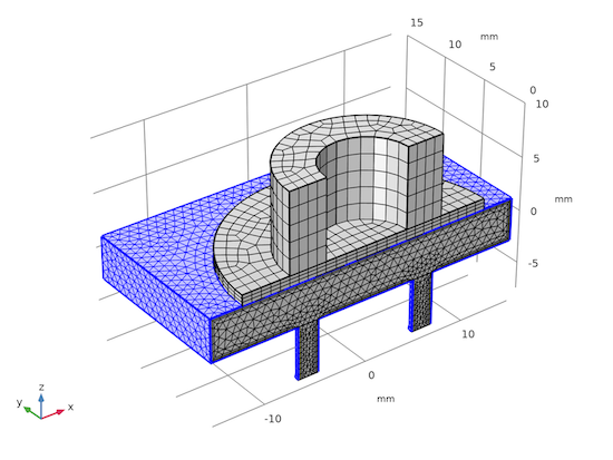
Consider an annular piezoelectric actuator with a circular membrane attached at the bottom, and the membrane in turn covers a fluid chamber with an inlet and an outlet pipe at its bottom. Mirror symmetry of the system allows only half of the geometry to be included in the model, as shown in Fig. 1.
The circumference of the membrane and the actuator’s top surface are anchored. A sinusoidal voltage is applied to the actuator. The piezoelectric stack expands under the applied voltage, which pushes the membrane into the fluid chamber. This forces out some of the fluid. After half of a driving cycle, the stack contracts and pulls the membrane upward, which draws fluid into the chamber. To direct the fluid flow, the two pipes have one-way valves installed such that fluid is drawn into the chamber through the left pipe and pushed out through the right pipe.
When creating a model to perform numerical simulation of a system, it is beneficial to ask what details should be included and what other details should be neglected or simplified. The simpler the model, the easier to set up correctly and the faster to compute. This model includes two simplifications.
The first is the piezoelectric stack. Instead of modeling it realistically as layers of piezoelectric material and electrical contacts, we choose to simplify the stack to a bulk block of piezoelectric material and apply to it an equivalent voltage to give the same electric field value in the material as in the layered structure. The stack is assumed to be composed of 75 layers of 100-um thick piezoelectric, and the applied field is 0.2 V/um. This leads to the equivalent applied voltage of 1500 V across the bulk block of piezoelectric, as shown in the table below. In a real device, the electric field and layer thickness determines the actual applied voltage.
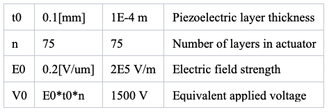
An example set of parameters relating the thickness and number of layers, as well as the electric field and equivalent voltage to be applied to the bulk block of piezoelectric.
The other simplification can be made regarding the one-way valves. The detailed working mechanism of such valves can be quite involved and is not the focus of this model. So we choose to represent the valve by a simple boundary condition and arrive at a much more efficient model. The boundary condition is based on the intuitive idea that the loss should be high when it flows against the valve and the loss should be low when it flows in the desired direction, the so-called K-factor piping losses. Specifically, the effect of the valve is captured by modeling the back pressure using this simple equation (1):
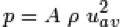
where A is a dimensionless number with a magnitude that depends on the flow direction, p is the fluid density, and u (av) is the normal component of the average velocity.
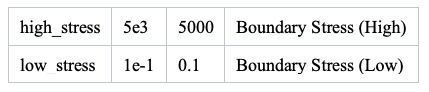
To minimize the effect of this somewhat artificial boundary condition on the flow pattern in the fluid chamber, two short pipes are added at the bottom of the chamber, as shown in Fig. 1. The boundary condition is applied at the end of each pipe to allow realistic flow to develop along the length of the pipe. The values for the number A ![]() for the two pipes are arranged in the opposite fashion so that one pipe serves as the inlet and the other as the outlet. The specific values for the high- and low-loss directions are 5000 and 0.1, respectively. These values are chosen to mimic a valve with low resistance (for example, a simple flapper valve). Obviously, these values should be tuned, and the formulation can be refined to make the model even more realistic when simulating a specific pump design.
for the two pipes are arranged in the opposite fashion so that one pipe serves as the inlet and the other as the outlet. The specific values for the high- and low-loss directions are 5000 and 0.1, respectively. These values are chosen to mimic a valve with low resistance (for example, a simple flapper valve). Obviously, these values should be tuned, and the formulation can be refined to make the model even more realistic when simulating a specific pump design.
COMSOL Multiphysics provides a graphical user interface with a Model Builder tree structure, the flexibility of customization with user-defined expressions and equations, and the versatility of many built-in multiphysics couplings. We will highlight these features by pointing out a few selected parts of the model. The full model and an accompanying PDF documentation with detailed instructions can be downloaded from the COMSOL website.
Continuing the discussion on the boundary condition for the inlet and outlet, the two values of A are first defined as global parameters, and then the dependence on the flow direction is easily entered as a user-defined expression in the input field for the back pressure, as shown in the parameter table and Figure 2.
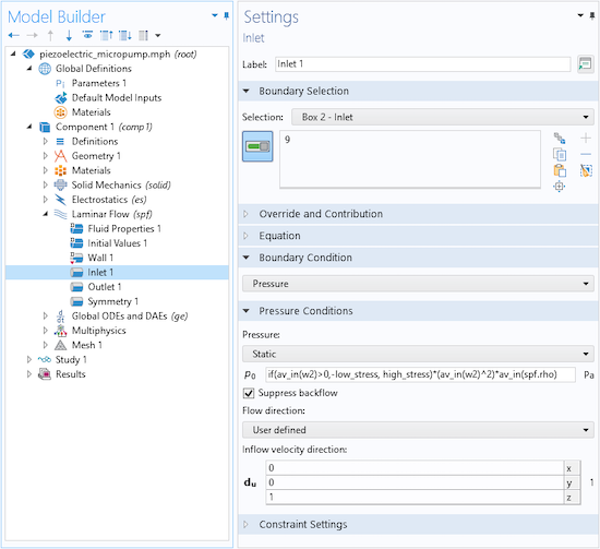
This flexibility of an input field being able to accept not just a number, but any parameter, variable or math formula, makes it straightforward and powerful to customize a model.
It is also easy to add user-defined equations. For example, in this model, two simple global ordinary differential equations are used to compute the cumulative flow through the inlet and outlet by integrating the flow rate over time.
As another example of the flexibility of the COMSOL software, consider the meshing of the solid and liquid domains. Each domain may be best suited for a particular kind of mesh, and the software handles disconnected mesh across the domain boundary seamlessly (no pun intended), as shown in Fig. 3. Note that the solid domains are filled with swept mesh and the fluid domain is instead filled with tetrahedral mesh with boundary layers highlighted in blue. At the solid–fluid interface in particular, there are unaligned mesh nodes on the solid and liquid sides.
The piezoelectric effect couples electrostatics with solid mechanics, and the deformation of the solid–fluid interface is accounted for by balancing the viscous, pressure, and inertial fluid forces on the membrane and the momentum transfer back to the fluid. Both of these fully bidirectional multiphysics couplings are easily implemented with built-in features in the software.
Once the model is computed, a full array of evaluation and plot features can be used to visualize the result in the same user interface. Fig. 4 shows the flow rates at the inlet and outlet (the blue and green curves), as well as the volume conservation, which is indicated by the net flow rate minus the rate of change of the volume of the chamber (the red curve). The applied voltage in the model is turned on from 0 up to the full strength during the first three-quarters of the drive cycle. Fig. 4 shows that soon after a time-periodic flow pattern is established.
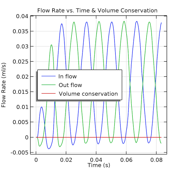
Fig. 4: The volume conservation and flow rate.
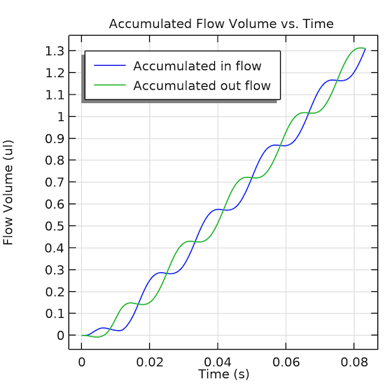
Fig. 5 shows the cumulative flow through the inlet and outlet as computed by the global equations. From the figure, we can read off the net flow value of 1.8 µL over a time period of 0.05 seconds, which corresponds to 36 µL/s or 2.16 ml/minute. This is consistent with typical values found in non-resonant pumps.
To show the pattern of the fluid flow during each half of the drive cycle, we plot the results at two separate instants in two sets of graphs (Figs. 6, 7). The first set shows the velocity field of the fluid and the solid. The second set shows the fluid streamlines. The graphs vividly display how the fluid is drawn into the chamber through the inlet at one instant and pushed out of the chamber through the outlet at the other instant.
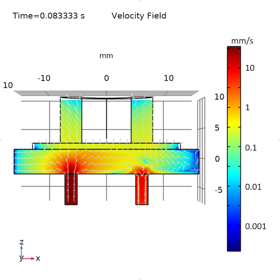

Fig. 6: The velocity field at an instant when the fluid is drawn into (left) and pushed out of (right) the micropump.
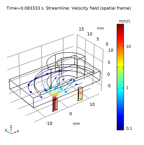
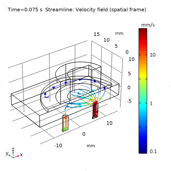
Fig. 7: The fluid streamlines at an instant when the fluid is drawn into (left) and pushed out of (right) the micropump.
We briefly discussed how a piezoelectric micropump can be efficiently simulated with reasonable simplifications and how the the COMSOL Multiphysics software make such simulations easy to perform. Modeling and simulation have become increasingly important in all sectors of industry.
Chien Liu is a Technology Manager at COMSOL, Inc.


COMSOL is a global provider of simulation software for product design and research to technical enterprises, research labs, and universities. Its COMSOL Multiphysics® product is an integrated software environment for creating physics-based models…

Ebook download: Powering Clean Energy Solutions
In this ebook, we explore 6 cases where modeling and simulation were used to help overcome these new design challenges. Topics include water turbines, sand-based heat storage, hydrogen fuel cells, and more.
Join over 90,000 engineering professionals who get fresh engineering news as soon as it is published.


About Us · Contact Us · Editorial Team · Advertising · Privacy Policy · Subscriber Services · © 2026 Digital Engineering 24/7 · Peerless Media